Architecture

General abstractions

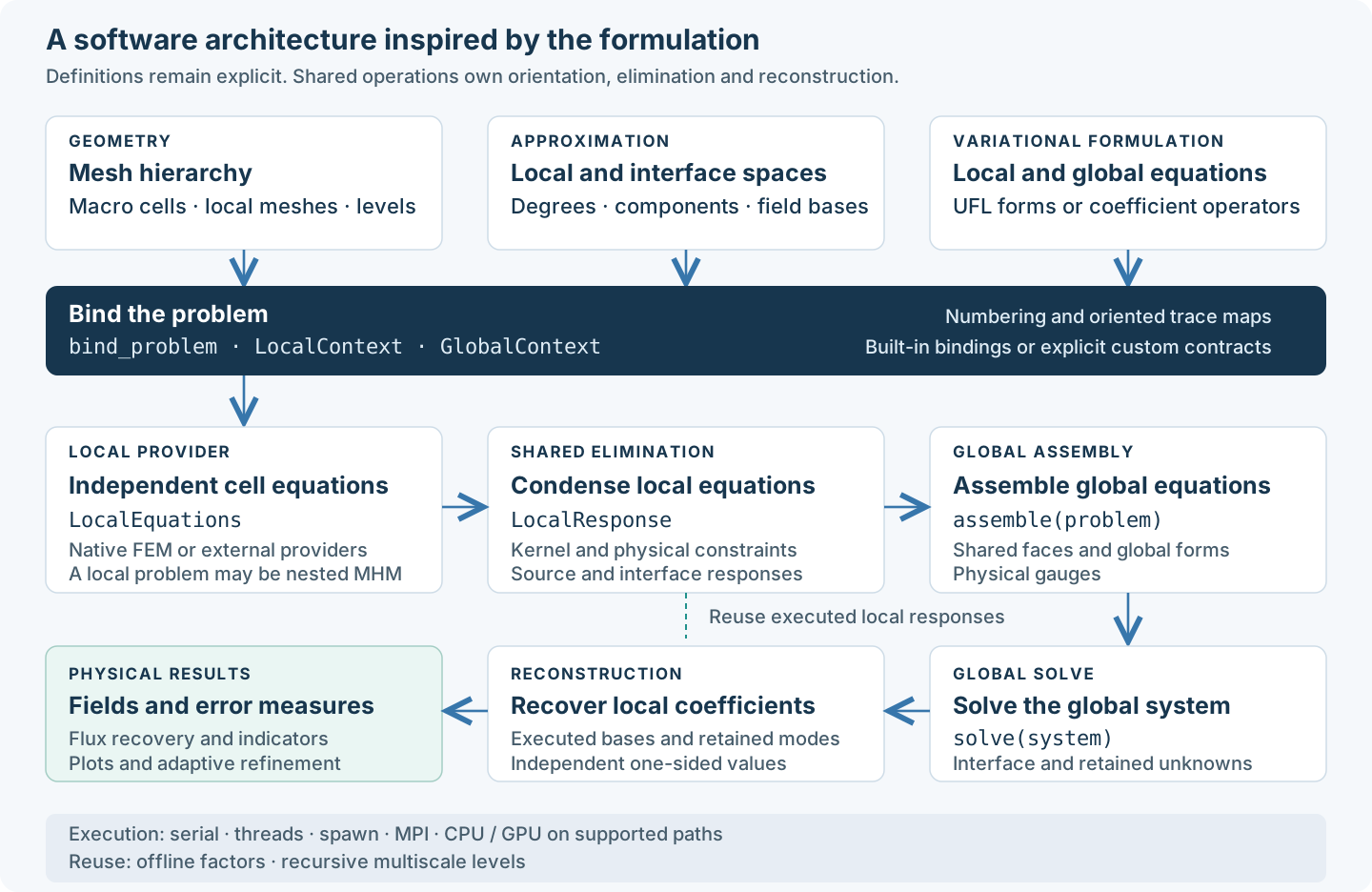
The user's workflow defines meshes and spaces, writes local and global equations, assembles, solves and evaluates physical fields. bind_problem connects those definitions to the shared multiscale operations. Built-in interface bindings provide numbering and orientation; custom spaces may supply their own declared maps. Physical boundary variables and the mathematical operator remain part of the user's equations.

A local provider supplies equations and ordinary field metadata. It can use UFL/DOLFINx, PyMHM's finite-element operations, an external solver or another multiscale problem. Condensation, ordered global reduction and reconstruction have shared owners. Execution and solver settings select supported backends without changing that mathematical interface; individual backends retain their documented space, matrix and platform restrictions.

The reconstruction uses the executed local responses and basis descriptors. Flux recovery and indicators consume the reconstructed fields; they can drive another refinement cycle. Offline factors reuse unchanged operators, and nested local problems repeat the same workflow at another scale.

Follow the feature overview for a first calculation, the method tutorials for formulations and the source-generated API for exact contracts.

Package responsibilities

The runtime is organized by numerical responsibility. Variational records, element assembly, hybrid elimination, execution and linear solves have independent owners. Predefined physical formulations compose these operations and preserve the established discretizations and field data contracts.

Package	Responsibility
core	Mesh/space bindings, variational contexts, local equations, condensation, reconstruction and global hybrid assembly.
fem	Basix reference elements, scalar/vector operators, H(div) spaces, traces and material quadrature.
meshes	Geometry, incidence, local submeshes and conforming refinement.
materials	Material laws, discontinuous coefficients and separable source fields.
_legacy.models	Predefined Darcy, flow, elasticity, transport and wave formulations.
methods	Robin MH, three-field MH²M, MsHHO and residual Petrov–Galerkin constructions.
recovery	Equilibrated and moment-based physical flux reconstruction.
estimators	Field indicators and error estimators with their stated admissibility conditions.
adaptivity	Marking, refinement decisions and adaptive solve policies.
linalg	Sparse factors, block solves and separable iterative operators.
execution	Ordered CPU batches, MPI assembly and accelerator execution.
backends	Optional native space bindings, trace/global form adapters, compilation and reusable workspaces.
io	Mesh/material exchange and executed-source fingerprints.
postprocessing	Named fields with their executed basis, evaluation and optional visualization.

The private _legacy.models subpackages contain the predefined physical solvers used internally by the verified cases. User-written problems use the generic variational interface. A geometry object stores topology and mappings; forms declare its physical operator, and a solver or estimator consumes the resulting operators without owning the basis construction. Scientific cases, manufactured data, campaign helpers and publication plots belong outside the runtime, with notebooks as their public entry points.

The root resolves exports on demand, and its __init__.pyi declares the typed generic variational and numerical API. __all__ and dir(pymhm) expose those same infrastructure names. Physical and method-specific operations are imported from their canonical submodules. Shared numerical operations likewise import their owners directly. The main problem-definition path binds MeshHierarchy, an interface space and user-written local/global forms with bind_problem. LocalContext and GlobalContext supply representation details. Fully explicit Equation, LocalEquations and MultiscaleProblem remain available; assemble and solve operate on both descriptions. The variational guide states their mathematical conventions and compilation limits.

Data and operations

Problem descriptions, execution settings, local responses and solutions are separate objects. Numerical operations are free functions; the existing LocalProblem, LocalResponse and HybridSystem methods delegate to the same implementations. Both interfaces use the same represented operators, oriented maps, executed retained bases and residual checks.

Responsibility	Objects	Functions
Bind mesh-associated problems	MeshHierarchy, BoundInterface, BoundProblem, LocalContext, GlobalContext	bind_interface, bind_problem
Declare custom coefficient conventions	InterfaceSpace, TraceBinding	bind_local_equations
Evaluate executed physical fields	FieldDefinition, DiscreteField	solution_field, evaluate_field
Describe local and global forms	Equation, LocalEquations	columns, rows, compile_form, compile_local_equations
Assemble a variational hierarchy	MultiscaleProblem, NestedEquations	assemble, solve
Reuse and recover an assembled hierarchy	MultiscaleSystem, MultiscaleSolution	with_global_load, with_global_equation, solve_multiscale_system, reconstruct_multiscale, leaf_moment
Describe fixed hybrid forms	LocalForm, GlobalForm, HybridProblem	compile_local_forms, assemble_hybrid, solve_hybrid
Execute independent cells	ExecutionConfig, callable provider	iter_local, map_local
Eliminate and reconstruct	LocalResponse, SolverConfig	condense_local, energy_reconstruction, local_condensation_system, reconstruct_local, reconstruct_response
Reduce and solve global equations	HybridSystem, HybridSolution	local_global_contribution, assemble_hybrid_contributions, solve_hybrid_system, hybrid_mean_constraint

Each formula has one owner. Offline factors, GPU batching, refinement and physical drivers reach that owner through object methods or the free functions. A factorization remains an object with an explicit lifetime; it owns native resources rather than defining the physical problem.

Within core, contracts owns validated coefficient records, condensation owns constrained local elimination, reconstruction owns recovered local coefficients, and contributions owns oriented sparse reduction. system combines these operations for the assembled problem; assembly coordinates ordered local providers. The classes in contracts and system store data and offer methods that delegate to these same free functions.

equations owns the four variational blocks, ordered trial/test trace maps and form compilation. multiscale composes those blocks with an additional global equation, ordered execution and recursive reconstruction. It delegates local elimination to the same numerical owners. moments owns reconstruction under declared physical moments; its saddle solve belongs to linalg.moments. The optional backends.forms adapter assembles user-defined UFL matrices and vectors; it selects no physical equation or boundary convention.

MultiscaleSystem.solve, reconstruct and with_rhs delegate to the corresponding free functions. A global load update reuses the executed local responses and their literal bases; retained source-compatibility rows remain unchanged. Changing a volume source requires new local equations or explicitly cached local factors. OfflineMultiscaleSystem owns those factors and updates volume sources, local balance loads and the additional global functional while preserving executed harmonic lifts, metadata and field maps. It is independent of a physical problem or time integrator. with_global_equation adds an independent operator and load after local responses are available, including an explicitly assembled jump of reconstructed fields. It returns a new system and preserves the executed bases and children.

Mesh-associated variational contexts

core.spaces owns portable interface maps and the structural custom-space contract. core.context binds macro/local meshes, user forms and declared retained dimensions to the existing MultiscaleProblem; it implements no new condensation or solver. A worker creates LocalContext for one macroelement, compiles the user's independent pairings and releases local native bindings. GlobalContext supplies interface boundary moments, selectors and supported native global forms. Geometric signs are transported once; physical signs and trial/test relations remain explicit.

backends.spaces binds supported portable meshes to user-selected native spaces. Nodal coordinate conversion uses incidence and Basix reference interpolation data. H(div)/H(curl) moment coordinates retain their declared native conventions. backends.traces binds supported edge and triangular traces and additional global interface UFL forms. Custom spaces may supply those capabilities independently; unsupported couplings fail explicitly.

postprocessing.fields associates reconstructed vectors with named fields, meshes, components, declared affine local/trace reconstructions and executed basis descriptors. Its free functions own evaluation and the solution's convenience field method delegates to them. Independent one-sided values are preserved.

ComponentTraceSpace preserves a scalar interface layout and interleaves Cartesian components. Tangential traces instead retain their declared physical frames. The general trace integration owner supplies Gram operators, linear functionals and projections in these same coordinates; it chooses no PDE or physical boundary variable.

Built-in bindings and fully manual definitions share the same numerical owners. See the overview for the principal workflow and custom interfaces for arbitrary numbering, dense basis changes and explicitly supplied maps.

The API qualification record compares the explicit and contextual providers for the main Darcy, SPE10, elasticity, MsHHO and MH²M examples. Both routes use the same current numerical owners and unchanged physical data. Coefficients are compared in a common physical basis; deterministic value and gradient samples additionally check the native Lagrange field views. These controls establish agreement for those examples, independently of their convergence and literature acceptance studies. Local RAD and Stokes–Brinkman controls cover both Galerkin and USFEM operators, boundary/interior macrocells and mild/extreme coefficients, including their source, trace-lift and retained responses.

Darcy formulations

Darcy providers compose the following public owners to distinguish approximation spaces and boundary variables. Their discretizations preserve their respective physical laws, spaces and coefficient conventions.

Owner	Local approximation and scope
fem.scalar.triangle, operators and tetrahedron	Conforming local scalar pressure on triangles or tetrahedra, coupled by a physical normal-flux skeleton.
fem.scalar.quadrilateral	Tensor-product local pressure on Cartesian macrorectangles.
fem.hdiv.rt_forms, rt_trace and mixed	Raviart–Thomas Darcy flux and discontinuous pressure, with hybrid or classical conforming assembly.
fem.hdiv.bdm_forms and mixed	BDM flux with the declared normal restriction and interior enrichment, coupled to discontinuous pressure.
fem.hdiv.mixed_3d, family_3d and mapped	Mixed spaces on affine tetrahedra/prisms or mapped hexahedra, with their stated Piola and moment conventions.
core.contracts, core.equations and core.subspaces	Explicit analytical local-response spaces and declared moment complements.
fem.scalar.quadrilateral and linalg.separable	Classical Cartesian reference assembly and reusable separable operators.
postprocessing.velocity	Conversion of supported Darcy fields into physical transport velocities.

Shared mixed assembly integrates supplied flux/divergence/pressure tables and constructs the normal-flux saddle in one owner. Element families supply their actual DOF maps, boundary moments and basis coordinates. They retain distinct normal degrees, pressure spaces, kernels and physical gauges; selecting a different family does not silently replace those contracts. See the scalar tutorials for the available variants and the Darcy API for their parameters.

Coefficient evaluation belongs to materials.evaluation: scalar, vector and SPD tensor fields use the declared point-major layouts and dimension-specific validation. fem.assembly.assemble_element_blocks scatters supplied dense blocks into the explicitly indexed row and column spaces. Repeated coordinates are summed during sparse conversion. Physical models supply their quadrature, coefficients and signed operators to these shared operations.

Variational descriptions and providers

The primary variational interface declares both local equations:

\[ \begin{aligned} a_K(u_K,v_K)+b_K(\lambda_K,v_K)&=L_K(v_K),\\ c_K(u_K,\mu_K)+d_K(\lambda_K,\mu_K)&=g_K(\mu_K). \end{aligned} \]

LocalEquations stores these independent blocks and their explicit trial/test trace maps. Equation supplies additional global bilinear and linear terms in the complete reduced coordinate order. MultiscaleProblem combines the forms, ordered local items, a callable provider, trace and retained dimensions, fixed coefficients and physical constraint rows. A local operator can be another MultiscaleProblem, with its reduced coordinates serving as the parent local basis. Recursive children leave boundary data and gauges to their parent. NestedEquations additionally constrains child boundary trace coordinates through an explicit oriented restriction and boundary reactions, using the shared core.nested operation.

A provider returns LocalEquations or CompiledLocalEquations. It can use assembled matrices, UFL/DOLFINx or another numerical package. The native compiler accepts real linear and bilinear forms, including distinct trial/test spaces, on single-rank meshes; local elimination needs a square local pivot. columns and rows describe signed linear trace pairings without requiring implicit cross-mesh assembly. Cross-mesh UFL integration requires explicit entity maps. The variational guide explains compilation, retained modes, recursive limits and method-specific space conditions.

LocalForm, GlobalForm and HybridProblem describe a fixed hybrid construction. LocalForm represents the local source and trace columns but does not declare independent trial/test pairings. GlobalForm describes the algebraic layout, boundary load and constraints of that construction; it is not an arbitrary global UFL form. Both interfaces delegate elimination and reconstruction to the same checked owners.

SolverConfig.local_solver accepts a callable on the constrained matrix and all source/trace/retained-mode right-hand sides. Every returned column must satisfy the unchanged original residual criterion before decoding. A response model must provide the operator, coordinates and complete response contract; its implementation does not establish approximation accuracy or stability. Portable metadata contains evaluation data, not live native meshes or factors.

Declared arrays preserve their stored precision. Native element tabulations and DOLFINx assembly use binary64; retaining wider correction digits through a solve requires the explicit extended refinement setting.

Local operators

LocalProblem(A, B, f, trace_dofs, kernel=Z, constraints=C) represents

\[ A_K u_K+B_K\lambda_K=f_K,\qquad u_K=w_K+Z_Kc_K,\quad C_K^T w_K=0. \]

The coupling already contains face orientation signs. The kernel is checked against A @ Z and A.T @ W, where left_kernel=W defaults to Z. Distinct left and right nullspaces are allowed when their respective constraint pairings are nonsingular. For L2 orthogonality use C=M @ Z. The represented floating-point actions of declared null modes are retained: nonzero A @ Z or A.T @ W uses the complementary response below. Only exactly vanishing represented actions permit the shorter kernel formula. Accumulation uses wider precision where available and compensated sums otherwise.

coarse_basis=Z instead retains modes that need not be null vectors, with the same nonsingular moment pairing. This prevents cancellation between large local responses when reaction or Brinkman drag approaches zero. The operator is not perturbed: the complementary solves include A @ Z, reconstruction uses E=Z-R @ A @ Z, and the global system retains the equations tested against Z. Here R denotes the constrained local solve. kernel and coarse_basis are mutually exclusive. The condensation API documents the nonsymmetric blocks and reconstruction of integral constraints.

A constrained factorization solves all source and trace right-hand sides together. LocalResponse stores the lifts. HybridSystem assembles sparse contributions, solves the global system and reconstructs every local field. The independent uncondensed block system is checked in tests to verify the signs of this process.

Geometry and trace spaces

TriangleMesh copies and orients its cells, rejects degenerate and nonmanifold connectivity, and records signed face incidence. SkeletonSpace accepts one FaceSpace for each face. Each FaceSpace has arbitrary increasing breaks in [0,1] and one degree per segment; bases are discontinuous Legendre polynomials. With continuous=True, a nodal polynomial basis shares values at segment endpoints within the same macroface. It does not identify endpoints belonging to different macrofaces. Vector components are interleaved within each basis mode. Constant traces are represented through constant_coefficients(), which accounts for the different basis conventions.

Boundary integration splits at both local mesh vertices and skeleton breaks. Thus local and skeletal partitions can differ for primal local spaces. Increasing trace dimension without enriching local spaces can violate the discrete inf-sup condition. Singular systems are errors; no diagonal shift or least-squares solve is used to conceal them.

PolygonMesh retains original macroedges while triangulating local domains, including simple nonconvex polygons. PolyhedralMesh represents convex and certified star-shaped nonconvex cells with planar polygonal faces. Shared face triangulations and cones from a certified interior point define local tetrahedra, while PolygonalSkeleton3D keeps one P0 or P1 space on each original face. Triangulating a quadrilateral face therefore does not introduce independent multipliers on its two triangles. The polyhedral RAD cases exercise cubes and two prism families; polygonal cases cover five planar families.

Mapped hexahedral RT fields use a trilinear geometry and contravariant Piola transformation, with surface Jacobians in normal moments and the physical Jacobian in divergence. Independent normal and interior degrees distinguish the rectangular enriched RT spaces from a uniformly raised polynomial degree. The well studies report geometric, normal-continuity and physical-rate checks separately from pressure and flux approximation.

Local backends

Reference-element libraries

pymhm.fem.reference delegates reference-element creation, values, Cartesian derivatives and entity transformations to Basix. ReferenceElementSpec uses the library's own family, cell, degree and variant names. create_reference_element records the native coefficient matrix after dualization, its digest, mapping, polynomial set and backend version. tabulate_reference supports the installed library's derivative orders and element shapes; it applies no physical Piola map or global face orientation. An explicit dof_ordering reorders both the archived coefficient matrix and the full orientation maps into the executed coefficient order. Entity-local maps keep their intrinsic order; reference_entity_dofs identifies their global slots in that executed order.

from pymhm.fem.reference import (
    ReferenceElementSpec, create_reference_element, tabulate_reference,
)

element = create_reference_element(
    ReferenceElementSpec("P", "triangle", 4, lagrange_variant="equispaced")
)
table = tabulate_reference(element, [[0.2, 0.3]], nderiv=2)

Basix supplies the built-in interval, triangular and tetrahedral Pk tabulations. Nodal permutations preserve PyMHM's topological numbering; affine Jacobians map Cartesian reference derivatives into physical coordinates. The public barycentric derivative representation uses the extension p(lambda_1,...,lambda_d), with zero lambda_0 derivatives, on the unit-sum hyperplane. Cartesian Qk bases use native interval factors in declared tensor order.

At literally declared interpolation nodes, nodal values equal their Kronecker rows. This applies the interpolation functional without a proximity threshold; nearby points and derivatives use the executed native tables. Tetrahedral face values use the exact topological support of the nodal trace. Compiled scalar diffusion kernels compensate Cartesian contractions and quadrature sums in binary64. Boundary moments also use compensated summation. Matrix entries, quadrature, coefficients and physical operators retain their declared conventions.

RT and BDM tabulations use native elements, transformed into the declared normal/interior moment coordinates. Basix RT degree one denotes mathematical RT0; simplicial BDM uses its vector polynomial degree. Restricted/enriched MHM spaces retain the stated normal restriction and all prescribed bubble modes. Their subspace maps, physical gauges, Piola transformations and face orientations remain explicit PyMHM responsibilities. Prism spaces use native simplex and interval polynomial factors. The persisted candidate-coordinate matrices retain their meaning during field replay.

Conventional Legendre moment tests and declared monomial coordinates delegate repeated value and derivative evaluation to Basix's orthogonal polynomial sets. Their normalization and representation maps preserve existing coefficient conventions. Exports of ascending-power coefficients are representation adapters for archives; they do not provide a second finite-element tabulator. Three-layer and elastic-wave archives record the executed native basis matrices. Persisted coefficient archives use their declared basis representations during replay.

Basix is a runtime dependency loaded at element creation or polynomial tabulation. DOLFINx, UFL, PETSc and MPI remain separate optional integrations. The algebraic local-provider and global-assembly contracts do not depend on a native element handle. The lockfile includes Windows packages; native execution checks in this workspace run on Linux. FIAT/FInAT can participate through a local provider or form compiler; a built-in FIAT adapter is not supplied.

Local finite-element assembly

The built-in FEM assembly uses Basix reference bases. FEniCS assembles the same LocalProblem from UFL forms. Arbitrary forms do not imply that their discretizations have been analyzed or benchmarked. In particular, H(div) normal boundary conditions are essential and require a correct lifting, restriction or augmented formulation.

The native RT0 implementation augments flux and pressure with local boundary pressure multipliers to prescribe normal flux from the MHM skeleton. It retains one joint constant-pressure/boundary-pressure null mode. It is a flux-based MHM local Neumann solve, not a pressure-trace hybridization relabeled as MHM.

The BDM2/P1 Darcy path uses the same flux-prescription principle with quadratic normal moments and a discontinuous linear divergence space. Its trace breaks must align with fine boundary edges. The mixed elasticity path uses a BDM2 stress row for each physical component, vector P1 displacement and scalar P1 rotation. Its retained rigid modes include the corresponding rotation multiplier, and its constraints are physical displacement moments. The enriched BDM and rectangular RT variants preserve their boundary normal degree while adding zero-normal interior fields; their displacement and rotation spaces follow the resulting divergence degree. See the mixed-family definitions and rectangular weak-symmetry construction.

Primal Darcy, conservative RAD and backward Euler use a shared nodal Pk tabulation, including physical gradients and Hessians. Displacement–pressure GaLS and equal-order flow use their complete strong residuals; prescribed coefficient derivatives enter the variable-material terms. A higher polynomial degree does not automatically validate an arbitrarily enriched trace space.

reconstruct_darcy_moments in pymhm.recovery.moments recovers RT0, RT1 or RT2 fields from skeletal, averaged interior-face and volume moments. Its source conservation is tested against continuous macro-local polynomials. equilibrate_flux instead adds fine-cell balance constraints to a minimum-energy RT0 correction. These reconstructions solve different mathematical problems. pymhm.estimators.darcy builds a separate conforming Oswald potential and evaluates the complete four-term energy estimator for identity diffusion. The fine meshes must join conformingly, and boundary and continuous-test moments are checked. Its explicit coefficient and boundary restrictions are part of the API; the recovery is never silently used to replace a plotted original field.

Independent checks use MSL_MHM with MSL_CG and MSL_Core for primal P1 local problems and NeoPZ for RT0/P0 mixed assembly. These comparisons match physical fields and trace spaces rather than assuming that internal basis coefficients or retained pressure coordinates have the same meaning in each implementation. The GaLS comparison also checks displacement, pressure, gradient and Cauchy stress against native MSL GaLS assembly.

Physical global gauges

Local constraints select complements during elimination; they do not replace physical global normalization. Pure-Neumann Darcy fixes one pressure mean. Pure-traction elasticity fixes all three planar rigid-motion moments. Flow pressure normalization depends on the boundary conditions and acts on the complete reconstructed pressure, including contributions from retained modes.

For flow with pure traction and no advection, a semidefinite resistance can leave only some translations unresisted. Automatic detection uses structurally zero material columns. A rotated nullspace can be supplied with translation_kernel; its independent columns are orthonormalized and checked against the material using a componentwise residual scale. mean_velocity cannot prescribe a resisted direction. A small positive coefficient is not silently replaced by zero.

For conservative RAD with zero reaction and divergence-free velocity tangent to the exterior boundary, a constant solution has an undetermined mean. Its discrete representation also requires the half-advection Robin multiplier to belong to the trace space. A continuous kernel alone does not imply a discrete kernel for an incompatible trace choice. Gauges are checked against the original assembled equations after solving.

Solvers and parallel execution

Global and local solvers are selected independently. All backends check achieved residuals, including multiple right-hand sides. SciPy and native direct backends reuse local factorizations. CPU workers preserve result order; process execution uses spawn on all platforms and limits native thread pools.

For SPD elliptic Neumann locals, AMG first projects each load onto the compatible range, pins independent kernel coordinates, solves the nonsingular principal system, and restores the physical mean. This preserves sparse matrices without a dense rank update. AMG is not blindly applied to the indefinite global saddle or to the local mixed Stokes/Darcy saddle matrices. The current AMG adapters reject a general coarse_basis; its augmented local system requires a supported direct solver. This restriction does not affect the AMG path for elliptic locals with a true constant kernel.

PDE drivers can pass assembled local operators to workers for condensation, or use a local factory to distribute assembly as well. solve_darcy and solve_darcy_bdm assemble in the coordinator by default; parallel_assembly=True constructs and condenses each macrocell in a worker. The RT and affine H(div) Darcy solvers, flow, displacement–pressure elasticity and conservative RAD use local factories. HybridSystem.from_local_factory(factory, items, ...) additionally distributes local construction and condensation together. Each worker calls the factory once and factors that local problem once for its source and all trace lifts. The parent assembles the global system from those completed responses.

A factory can return LocalProblem alone, or LocalAssembly(problem, metadata). The latter carries ordinary application data such as a local mesh or DOF map; system.local_metadata preserves input order. Returning the mesh built in the worker avoids rebuilding it sequentially for field reconstruction. This metadata does not change the variational operator or the condensation algebra.

Process execution uses portable spawn, so the factory, inputs, and metadata must be picklable. Construct and release native FEM, MPI, PETSc or CUDA resources inside the worker, returning numerical arrays and ordinary metadata. The serial and thread variants also accept closures. Exceptions propagate to the caller; there is no automatic serial fallback. The global assembly and solve remain in the parent process. See the measured workloads for costs of startup, data transfer, local work, and the complete solve.

solve_distributed provides a separate MPI path: ranks own local cells, PETSc owns global matrix rows, and MUMPS solves the distributed saddle matrix. OfflineHybridSystem retains local/global factorizations for changing sources and boundary values at a fixed operator. LocalFactorCache also reuses factors across exactly identical constrained matrices.

GPU sparse direct solvers upload CPU matrices. The explicit batched GPU API also provides resident affine P1 volume assembly and dense batched LU with multiple RHS. condense_multi_gpu assigns bounded local batches to explicit devices and uses sparse cuDSS for larger systems. Responses and ordinary skeleton assembly return to the host; the separate MPI path owns distributed global rows. See execution contracts and measurements.

Extension contract

A new local formulation supplies its matrix, signed trace forms, load, kernel and physical moments. Test its kernel and compatibility independently; then compare condensed and uncondensed solutions. Add PDE patches, independently derived sources, convergence and conservation diagnostics before adding a support claim.