Acoustic propagation in Marmousi II

A 20 Hz point source generates a complex pressure field in a heterogeneous geological model. This frequency-domain application uses a declared crop of the primary Marmousi II velocity and density data, with material interfaces resolved by the local meshes.

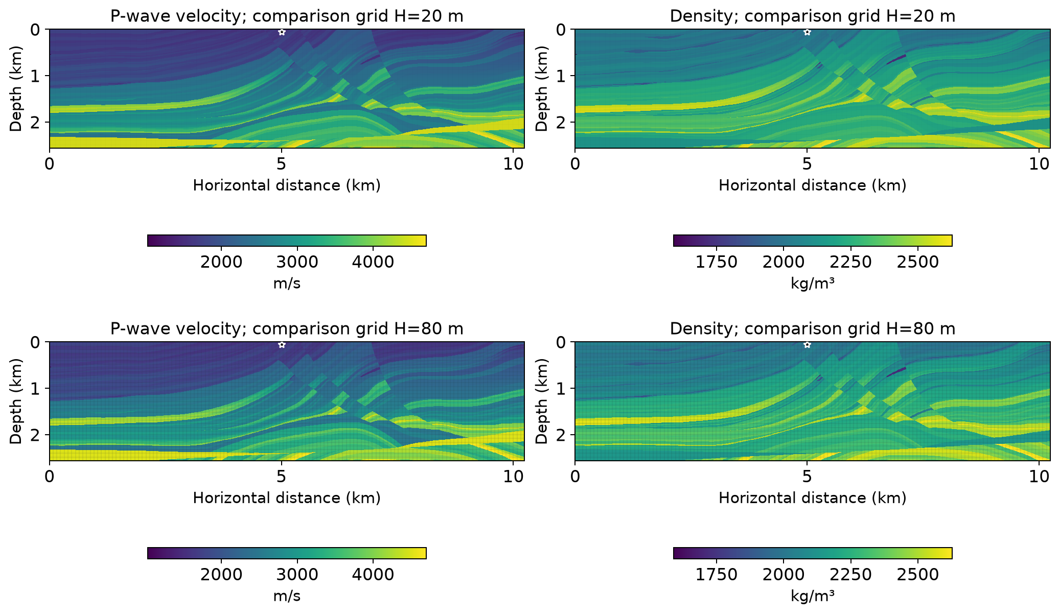
The top row overlays the comparison grid with \(H=20\) m; the bottom row overlays the grid with \(H=80\) m. The left column shows P-wave velocity in m/s, and the right column shows density in kg/m\(^3\). Both rows use the same material samples; only the overlaid grid changes. The white star marks the acoustic source. These panels describe the physical material used in the pressure equation.

Physical problem

Horizontal distance \(x\) and depth \(z\) are in metres. With density \(\rho\), sound speed \(c\) and bulk modulus \(\kappa=\rho c^2\), the equation is

\[ \begin{aligned} \Omega&=(0,10240)\times(0,2560),\\ -\nabla\cdot(\rho^{-1}\nabla p) -\omega^2\kappa^{-1}p&=\delta_{(5000,50)},\\ \omega&=2\pi(20\ {\rm Hz}). \end{aligned} \]

The top has \(p=0\). The remaining sides impose outgoing impedance:

\[ \rho^{-1}\partial_n p -\mathrm i\omega(\rho\kappa)^{-1/2}p=0. \]

The selected \(2048\times512\) material cells have width 5 m and crop origin \((3395,515)\) m in the primary data. Each cell value is a primary sample, without interpolation or averaging. Density and velocity are converted to kg/m\(^3\) and m/s before computing \(\kappa\).

Multiscale formulation and implementation

The executed MHM field uses \(512\times128\) macroquadrilaterals of width \(H=20\) m, local continuous \(Q_3\) on \(8\times8\) fine quadrilaterals, and linear conormal traces. There are 261,888 free complex trace unknowns.

Inside each macroelement, the volume form is

\[ a_T(p,v)=\int_T\rho^{-1}\nabla p\cdot\nabla\overline v -\omega^2\int_T\kappa^{-1}p\overline v -\mathrm i\omega\int_{\partial T\cap\Gamma_A} \frac{p\overline v}{\sqrt{\rho\kappa}}. \]

The local equation adds the oriented normal-flux trace pairing on active faces. The global equation sets pressure-jump moments to zero on interior faces and prescribed-pressure moments on the top. Absorbing flux follows the impedance condition; it is not an independently prescribed zero flux. The point functional is evaluated at its physical location. Since this source lies on a macroface, each incident macroelement receives half its unit strength.

The application's provider builds the complex form and passes its exact real/imaginary embedding to the generic equation API:

matrix = stiffness - omega**2 * mass
# Outgoing boundary integrals are included in matrix before this declaration.
coupling = sparse.kron(pairing, sparse.eye(2)).toarray()
local_equations = LocalEquations(
    a=realify_operator(matrix),
    L=realify_vector(load),
    b=coupling,
    c=-coupling.T,
    dofs=skeleton.cell_dofs(cell),
    g=-realify_vector(boundary),
)

See the Helmholtz method tutorial for the local/global derivation and the Marmousi notebook for data preparation, a smaller full-crop solve and the complete-study option. The default notebook configuration and the large acquired calculation have different approximation spaces; both are stated explicitly.

Results and reproducibility

An independent DOLFINx/UFL conforming reference is refined from \(P_1\) to \(P_4\) on the fixed 5 m material mesh. This is a polynomial-degree refinement control; a sequence of finer conforming meshes is not included. Its last global pressure L2 increment is 0.0786%; the MHM/P4 pressure difference is 2.6935%. Derivative comparisons exclude the fixed \(50\times50\) m square containing the singular source; the MHM/P4 acoustic-flux difference on that domain is 3.0369%.

These are differences from a refined numerical reference, not exact errors. The selected data are not identified with the historical coefficient arrays in the method article, so this application does not claim a literal reproduction of its table. The full report provides source URLs, checksums, norm definitions, original-equation checks and the acquisition/replay commands.

References

• Gary S. Martin, Robert Wiley and Kurt J. Marfurt (2006). Marmousi2: An elastic upgrade for Marmousi. DOI: 10.1190/1.2172306.
• Théophile Chaumont-Frelet and Frédéric Valentin (2020). A Multiscale Hybrid-Mixed Method for the Helmholtz Equation in Heterogeneous Domains. DOI: 10.1137/19M1255616.