MsHHO in three dimensions

solve_mshho_3d constructs cell and face moments on tetrahedral or convex polyhedral macro meshes. The local field minimizes physical diffusion energy subject to these moments. Local volume moments are condensed before the global face-pressure moment solve. MsHHO is the macro discretization, while the local energy reconstructions use conforming tetrahedral finite elements on fine submeshes. The implemented local discretization is not an HHO method on a second mesh. It uses the same projected-source and reconstructed-source conventions as the two-dimensional implementation, following Chaumont-Frelet et al. (2022). The article proves equivalence for its ideal local reconstruction spaces. Generic finite local meshes approximate those spaces; algebraic reconstruction alone does not establish the hypotheses of the paper's error estimates. The cases below use an analytical solution rather than a published numerical benchmark table.

Geometry, moments and boundary conditions

Each tetrahedral face carries independent \(P_\ell\) moments, optionally on an aligned triangular partition. Polyhedral faces retain moments on the original polygon, rather than independent traces on the triangles used to integrate it. Volume moments use \(P_m(K)\). The energy lift uses a conforming tetrahedral \(P_k\) local mesh, which must have enough independent degrees of freedom to represent all moment constraints.

Prescribed pressure is imposed through exterior face moments. neumann prescribes physical outward Darcy flux on selected faces. For pure Neumann data, compatibility is checked and mean_pressure selects the physical volume mean. The global mean is not a coordinate-dependent choice of one nodal value.

The example helpers below are repository sources, supplied separately from the installed library. Open the corresponding notebook to acquire its verified companion, as described in the notebook guide.

from pymhm import TetraMesh
from examples.formulations.application import moment_diffusion as solve_mshho_3d

solution = solve_mshho_3d(
    TetraMesh.unit_cube(2), source=1.0, degree=2,
    cell_degree=0, local_refinement=2,
)

source_variant="projected" uses the cellwise \(L^2\) source projection. source_variant="reconstructed" applies the original source to reconstructed test functions. Their fields coincide for represented polynomial sources. The face-only choice cell_degree=-1 requires the reconstructed-source variant. Tests cover both conventions, mixed and pure Neumann boundaries, tensor diffusion and source compatibility.

Exact local spaces for the selected constant-moment cases

For identity diffusion and constant volume/original-face moments, Equation (2.19) defines local functions with constant Laplacian and constant normal derivative on every original face. On a tetrahedron \(T\) and an axis-aligned box \(Q\), respectively, these spaces are

\[ \begin{aligned} \mathcal U^{0,0}(T) &=\operatorname{span}\{1,x,y,z,x^2+y^2+z^2\},\\ \mathcal U^{0,0}(Q) &=\operatorname{span}\{1,x,y,z,x^2,y^2,z^2\}. \end{aligned} \]

Compatible constant Neumann data and the constant kernel give dimensions five and seven. The volume and face integrals determine each polynomial uniquely: integration by parts gives zero energy for a polynomial whose moments all vanish, and the zero volume moment fixes its constant part. The same calculation makes each polynomial energy lift orthogonal to every fine finite-element function with zero moments. A conforming local P2 space contains these polynomials, so its energy lifts coincide with the ideal lifts for these particular geometries and \(K=I\).

The ten-case acquisition compares every column of the executed lift with this independent polynomial characterization. Its maximum relative discrepancy is \(5.890\times10^{-15}\); the executed matrix and field coefficients are retained. This exact-space argument requires local degree at least two and does not extend to degree one, higher moment degrees, general polyhedra or different materials. Those configurations can admit finite algebraic reconstructions without satisfying this argument.

Five-level unit-cube study

The material is \(K=I\), pressure is zero on the boundary, and

\[ p=\sin(\pi x)\sin(\pi y)\sin(\pi z),\qquad q=-\nabla p,\qquad f=3\pi^2p. \]

Both families use constant cell/face moments, local \(P_2\), and the projected source. Tetrahedral macrocells use local refinement two; cubic macrocells use their conforming tetrahedral decomposition at refinement one. These are different local meshes, so their errors are not an equal-cost comparison. The macro resolutions are \(n=1,2,3,4,5\). Assembly order nine and independent error rules ten and twelve give a maximum relative norm difference \(3.588\times10^{-10}\). The local refinement is an integer subdivision factor: each tetrahedral macro has eight fine tetrahedra, and each cubic macro has twelve. The executed coefficient precision is explicitly extended; native sparse factors use binary64. The default solver precision is documented separately from this acquisition setting.

Here \(n\) counts equal intervals along each side of the unit cube. The macro partition therefore has \(n^3\) cubes or \(6n^3\) tetrahedra: at n5, 125 cubes or 750 tetrahedra. It is independent of the local subdivision factor and polynomial degree. P2/P0 in these records denotes local pressure degree two and constant cell/original-face moments.

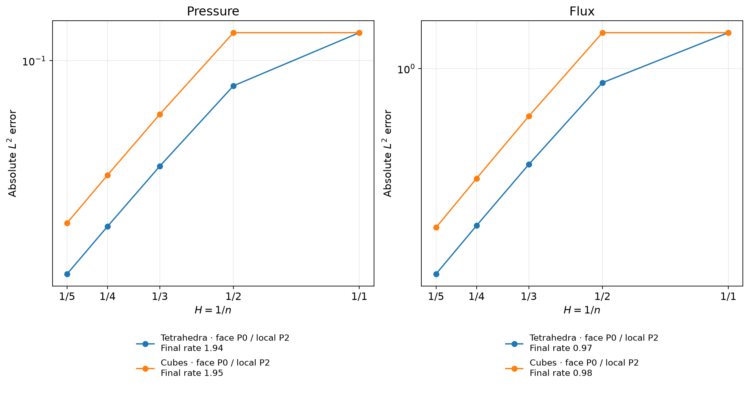
Macro geometry	Pressure L2 error at n=5	Final rate	Raw flux L2 error at n=5	Final rate
Tetrahedra	1.43723e-2	1.942	3.98453e-1	0.972
Cubes	2.28545e-2	1.954	4.90777e-1	0.984

The measured rates approach second order for pressure and first order for flux. Theorem 6.3 supplies a first-order energy estimate here: the smooth source satisfies \(f\in H^1\) and the exact flux satisfies \(K\nabla p\in H^1\). The second-order pressure rate is an observation from this study, rather than an additional consequence of that energy bound. The displayed flux is the raw physical field \(-K\nabla p_h\), with no separate H(div) postprocessing. Generic finite lifts do not guarantee H(div) conformity or fine-cell conservation. Conservation for a projected source refers to its macro P0 projection, not to the original nonconstant source at each fine cell.

For the selected identity-material tetrahedral and cubic P0 cases, the polynomial characterization above gives a stronger conclusion. The raw flux has constant divergence equal to the macro P0 source projection and constant normal trace on each original macroface. Global face equations match these normal traces with opposite outward orientations, so this particular flux is H(div)-conforming without postprocessing. Independent one-sided derivative checks on all ten acquired meshes confirm the divergence, fine-face normal continuity and macroface multiplier identity; their maximum scaled discrepancies are below \(5.889\times10^{-13}\). This statement concerns the projected source and these exact local spaces, not arbitrary finite local lifts.

The maximum relative residual of the original projected-source equations is \(5.789\times10^{-17}\), separately from approximation accuracy and uniform inf-sup stability. Actual volume/face moments, reconstructed matrices, raw energy matrices, physical maps, coefficients and cardinal value/derivative tables are archived. Original stiffness matrices in the archive are explicitly identified as diagnostic reassemblies by the shared operator owner.

An independently assembled FEniCS Basix 0.9.0 P2/P0 reference solves the same projected-source problem on all ten macro meshes. Both fields are evaluated with their own executed bases and physical maps. The maximum relative differences are \(1.327\times10^{-14}\) for pressure, raw gradient, physical Darcy flux and full broken H1 norms, and \(8.771\times10^{-15}\) for the physical P0 normal multiplier. Inserting the acquired coefficients into the original reference equations gives at most \(2.559\times10^{-14}\), against the unchanged \(10^{-10}\) criterion. Twenty data-only replays with one and two BLAS threads are bitwise identical. The reference independently constructs operators, moments, source projection and field norms; it shares the attributed SciPy factorization and original-residual arithmetic. Project, module, revision, verified source URL, runtime digests and all archive identities are in the independent verification record.

Sections and components

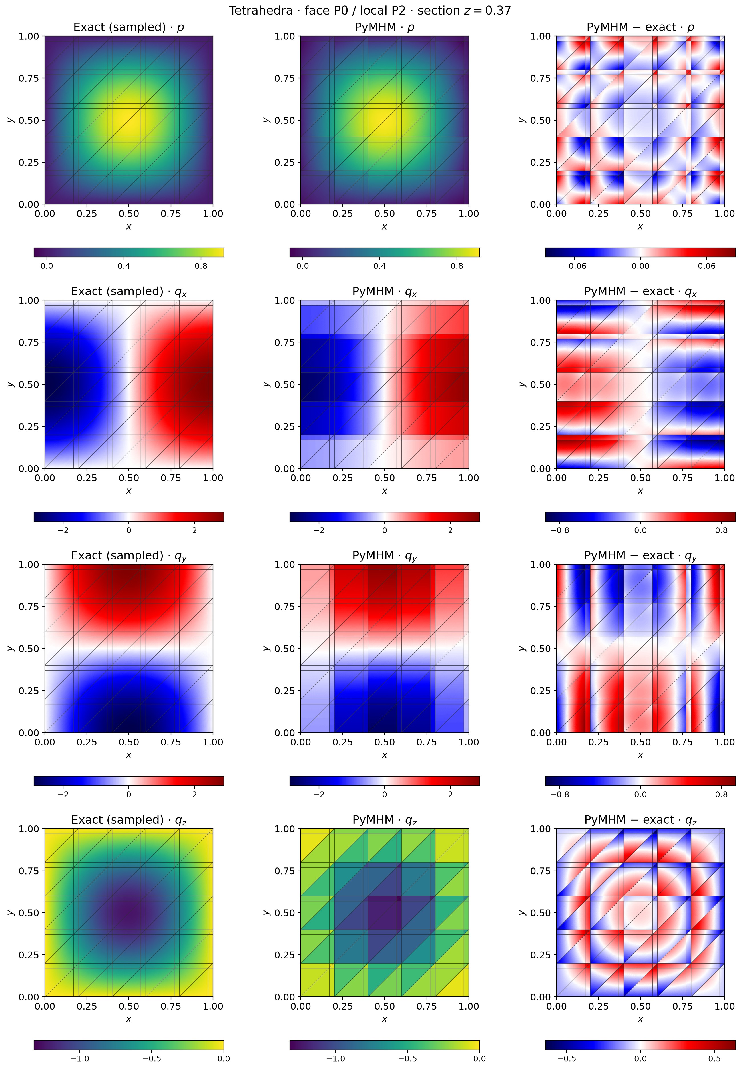
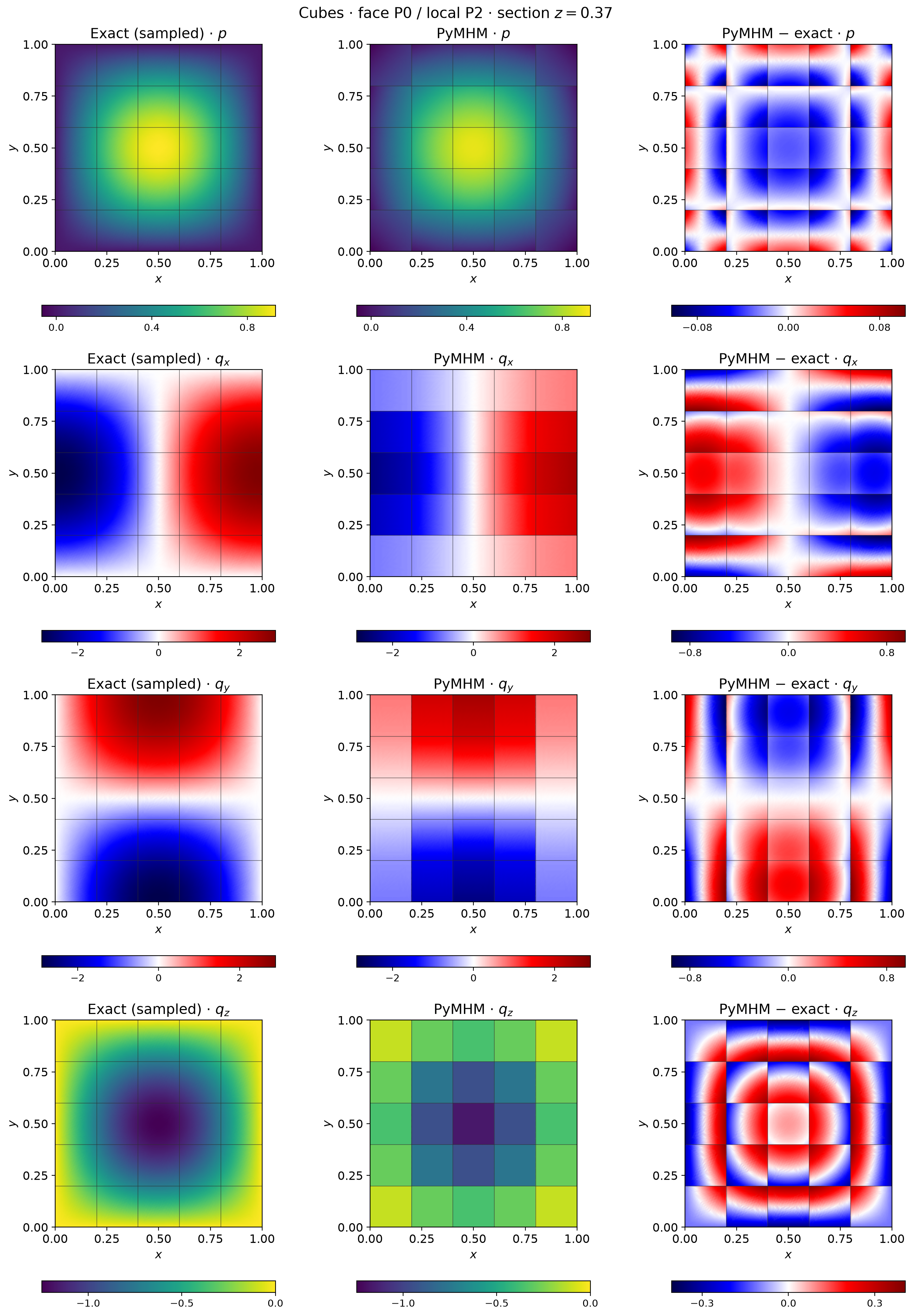
The section \(z=0.37\) displays the complete local pressure polynomial and every physical flux component. Exact and numerical samples share scales, while differences have independent symmetric scales. Original macroface intersections are overlaid. Each triangular fan of a fine-cell section has six display subdivisions; vertices remain private to their fine cell so that interpolation cannot smooth independent traces across interfaces. Both finest states are replayed and their volume error norms checked against the campaign before all local coefficients and section samples are archived.

pixi run --locked -e notebooks python -m examples.solve_core_extensions mshho3d
pixi run --locked -e notebooks python -m examples.sample_core_sections mshho3d
pixi run --locked -e notebooks python -m examples.plot_core_extensions mshho3d

The ten-case record is examples/results/core-extensions/mshho3d.json, with source hashes, error quadrature checks and section archives. The coefficient replay and display hashes are recorded separately in examples/results/core-extensions/mshho3d-field-sampling.json.

References

• Théophile Chaumont-Frelet, Alexandre Ern, Simon Lemaire, and Frédéric Valentin (2022). Bridging the Multiscale Hybrid-Mixed and Multiscale Hybrid High-Order Methods, ESAIM: M2AN 56, 261–285. DOI: 10.1051/m2an/2021082.