Recursive MHM local problems

An MHM discretization can supply a local problem at the next scale. This multilevel interpretation appears in Harder, Paredes and Valentin (2013), Remarks 7 and 10, and the local variational decomposition of Harder and Valentin (2016), sections 2 and 4.1. The current study is an original recursive realization on a declared Cartesian mesh. It compares recursive and flat MHM with identical leaf spaces, and verifies both against an independently assembled complete original Q2/P1 hybrid system.

Local equations and physical moments

Let \(A_{\mathrm{in}}x=b_{\mathrm{in}}\) denote the inner hybrid system, including its retained local modes. The columns of \(P\) select the inner boundary trace. The signed injective map \(T\) restricts the parent trace to that boundary. The parent local problem is

\[ \begin{bmatrix} -A_{\mathrm{in}} & P\\ P^T & 0 \end{bmatrix} \begin{bmatrix}x\\\mu\end{bmatrix} +\begin{bmatrix}0\\-T\end{bmatrix}\lambda =\begin{bmatrix}-b_{\mathrm{in}}\\0\end{bmatrix}. \]

Thus \(P^Tx=T\lambda\). The reaction \(\mu\) is minus the inner pressure moment; the parent pairing \(-T^T\mu\) preserves the continuity sign. NestedLocalProblem uses the shared LocalProblem condensation. Physical constant kernels, source offsets and moment constraints survive the second elimination. The executed retained basis \(E\) is archived separately from the selector \(P\), and field replay uses that same numerical basis.

nested_trace_map checks exact facewise representability and includes normal and parameter orientations. Each parent face has two independent P1 segments, exactly matching the two inner boundary faces. This restriction is a signed permutation; no projection or averaging changes the trace space.

Physical problem and finite spaces

On \(\Omega=(0,1)^2\), the permeability is \(K=I\). The two problems share the same independently derived source:

\[ \begin{aligned} p_0(x,y)&=\sin(\pi x)\sin(\pi y),\\ p_1(x,y)&=1+x-y+\sin(\pi x)\sin(\pi y),\\ f(x,y)&=-\Delta p_i(x,y) =2\pi^2\sin(\pi x)\sin(\pi y). \end{aligned} \]

Exact pressure is imposed weakly on every exterior face: zero for \(p_0\), and \(1+x-y\) for \(p_1\). No extra physical mean is imposed on this Dirichlet problem. The physical Darcy flux displayed here is \(q=-\nabla p_h\), evaluated independently on each leaf. It is a raw polynomial gradient, distinct from an H(div) reconstruction and from the oriented normal-flux multiplier on macrofaces.

For \(n=1,2,4,8,16\), the outer mesh has \(n\times n\) rectangles of size \(H=1/n\). Each contains \(2\times2\) inner macrocells, and each inner macrocell contains \(2\times2\) fine quadrilaterals. Continuous Q2 on each inner submesh has 25 nodal coordinates. Inner faces carry \(P_1=\operatorname{span}\{1,2t-1\}\), with canonical face parameter \(0\leq t\leq1\).

The local volume stiffness kernel is the declared physical constant, paired with its physical volume integral. Eight disjoint fine-edge midpoint functions provide a rank-eight witness for the local trace coupling: each face of length \(L\) contributes the block

\[ \frac{L}{3} \begin{bmatrix}1&-1/2\\1&1/2\end{bmatrix}, \qquad \det=\frac{L^2}{9}>0. \]

Trace continuity connects the leaf constants, and exterior Dirichlet data fixes the remaining global constant. This establishes finite-case injectivity and the physical gauge for these executed spaces. The single-polynomial Pk degree conditions of Lemma 10 in the cited chapter do not automatically apply to Q2 on a fine submesh. This study does not establish a mesh-uniform inf-sup estimate or transfer the chapter's convergence theorem to these spaces.

Measured fields and convergence

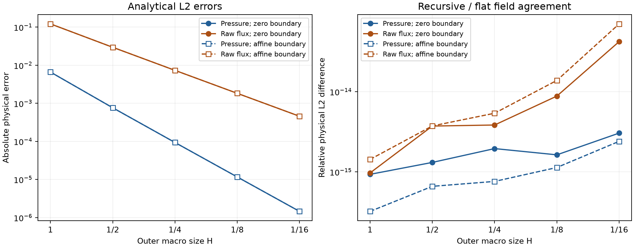
The analytical errors use physical leafwise integration. The raw-flux error is the gradient error because \(K=I\). The complete broken H1 norm also reported by the independent reference includes the pressure L2 term:

\[ \begin{aligned} \|e_p\|_{0,\Omega}^2 &=\sum_{K}\int_K |p_h-p_i|^2\,dx,\\ \|e_q\|_{0,\Omega}^2 &=\sum_{K}\int_K |q_h+\nabla p_i|^2\,dx,\\ \|e_p\|_{1,\mathrm{broken}}^2 &=\|e_p\|_{0,\Omega}^2 +\sum_{K}\int_K |\nabla(p_h-p_i)|^2\,dx. \end{aligned} \]

The public acquisition uses a six-point tensor Gauss rule per fine cell; weak boundary data uses eight points per face segment. Separate eight- and ten-point rules check all integrated errors and physical field differences. The maximum relative change between these two norm rules is \(3.69\times10^{-12}\).

Outer divisions	Recursive unknowns	Flat unknowns	\(\lVert e_{p_0}\rVert_{0,\Omega}\)	\(\lVert e_{q_0}\rVert_{0,\Omega}\)	\(\lVert e_{p_1}\rVert_{0,\Omega}\)	\(\lVert e_{q_1}\rVert_{0,\Omega}\)
1	17	28	6.60653e-3	1.21651e-1	6.60653e-3	1.21651e-1
2	52	96	7.62088e-4	2.95357e-2	7.62088e-4	2.95357e-2
4	176	352	9.32881e-5	7.31711e-3	9.32881e-5	7.31711e-3
8	640	1344	1.16000e-5	1.82493e-3	1.16000e-5	1.82493e-3
16	2432	5248	1.44810e-6	4.55957e-4	1.44810e-6	4.55957e-4

The final \(8\to16\) refinement gives measured pressure order 3.001892 and raw-flux order 2.000869 for both boundary problems. These are observed rates for the current smooth analytical family. The relative physical L2 difference between recursive and flat pressure or raw flux is at most \(7.01\times10^{-14}\); the maximum source-normalized original equation or constraint residual is \(6.64\times10^{-13}\). Macroface normal-flux equilibrium does not establish fine-cell conservation of the raw gradient.

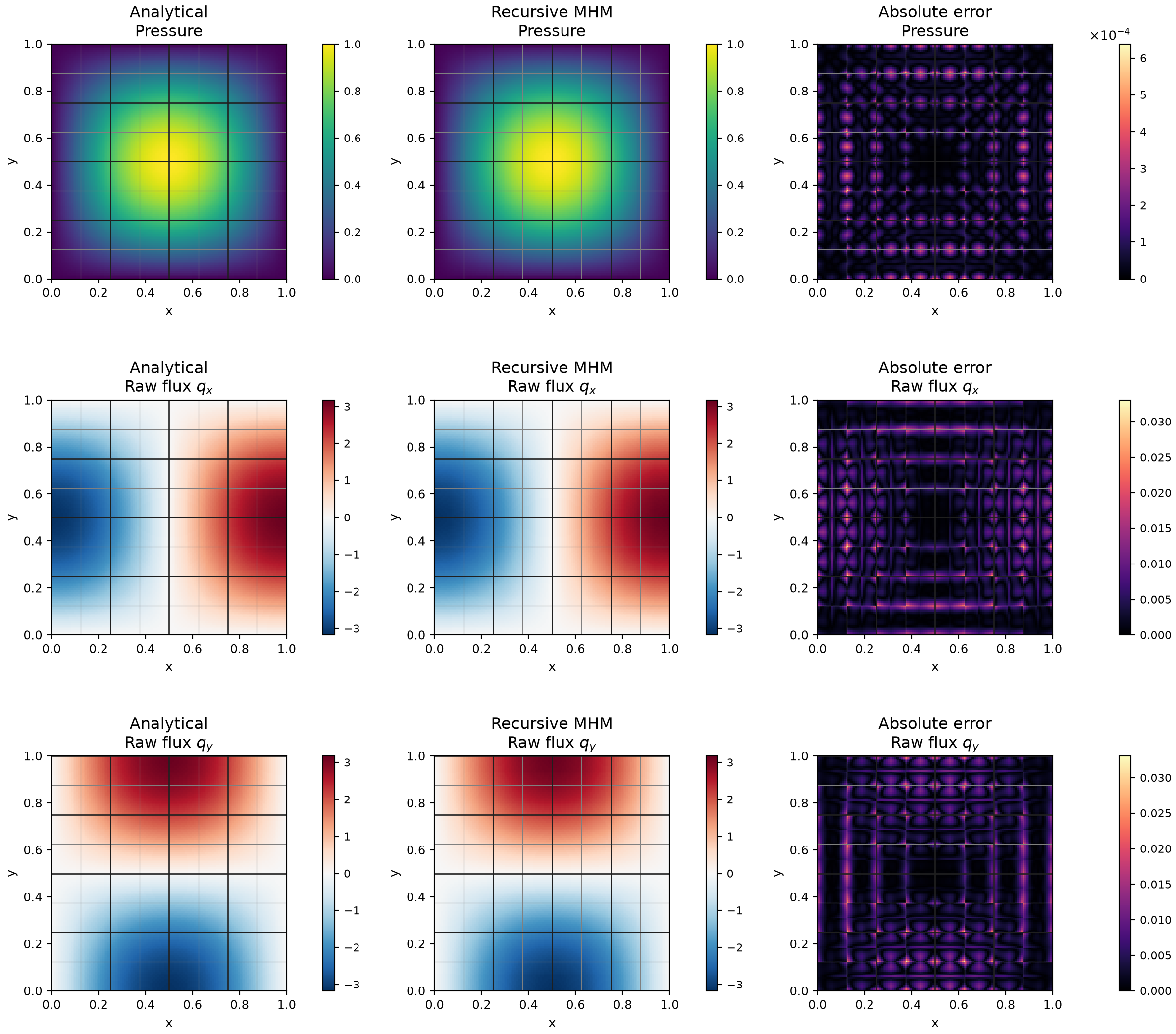
The spatial figure uses the homogeneous \(n=4\) acquisition. Every analytical, numerical and error panel marks the actual archived outer macrofaces in dark lines and inner macrofaces in thin lines. Saved one-sided field samples remain independent at interfaces; no smoothing or averaging is applied. Each panel has its own colorbar. Pointwise figure errors complement the integrated norms.

Independent original-system comparison

The executed reference uses FEniCS Basix 0.9.0, module create_element/tabulate, for independent equispaced Q2 and P1 basis tabulation. The upstream tag resolves to 19555f5b629b4090b14014f9db5f2c9ac80984f9. Compiled runtime digests are recorded separately; no byte identity to this upstream source checkout is asserted. An instrumented comparison assembly constructs the complete original Q2/P1 saddle system on the same geometry, coefficients, source, boundary data and approximation spaces. This is an executed assembly comparison, not an original author application or a classical conforming reference. It shares the attributed SciPy SuperLU factorization and extended original-residual policy, while geometry, basis, operator assembly and physical evaluation are independent of PyMHM assembly and condensation.

The native reference uses six Gauss points for both volume and face assembly; the affine weak Dirichlet moments are integrated exactly by this rule. Its field norms use the separate eight- and ten-point rules.

Both recursive and flat candidate fields are inserted into the independently assembled original equations. Pressure, raw gradient, Darcy flux, full broken H1 and the physical normal-flux multiplier are compared through physical norms on the same leaves or faces. Trace coordinates are transformed using actual endpoints, normals and parameter directions, without averaging. Across all ten complete cases:

Verification	Maximum relative value	Acceptance criterion
Native original equations	8.76e-13	1e-10
Candidate in native original equations	2.02e-12	1e-10
Physical fields and oriented normal multiplier	1.36e-12	1e-9
Represented A, B, source and weak boundary load	4.51e-16	1e-11
Native norm quadrature sensitivity	3.69e-12	1e-9

Twenty data-only replays and twenty physical comparisons produce bitwise identical results with one and two BLAS threads. The reference's final pressure, raw-gradient and complete broken H1 orders are respectively 3.001892, 2.000869 and 2.000891. Executed basis matrices, operators, field coefficients, producer and consumer identities have separate digests in examples/results/nested-current/native-verification.json.

The public acquisition took 155.46 seconds with 663.64 MiB peak owned RSS; its separate read-only archive closure took 81.71 seconds with 814.33 MiB. The complete native acquisition, comparisons and replays took 246.91 seconds with 630.27 MiB under overlapping host workloads. Costs include setup, serialization, synchronization and verification. Fewer outer unknowns measure condensation; these measurements do not demonstrate a runtime speedup.

Reproduction and archived evaluation

examples/results/nested.json selects the ten current acquisitions and their checksummed companion records. Numerical archives contain the actual original operators, retained bases, geometry, quadrature tables and one-sided display tables. They are generated locally and remain outside release artifacts. The plotting driver consumes these saved tables without solving or tabulating a new numerical basis:

pixi run --locked -e notebooks python -m examples.verify_nested \
  --levels 1 2 4 8 16 --boundary both --native-threads 1 \
  --acquire-only --output examples/results/nested-regenerated
pixi run --locked -e notebooks python -m examples.plot_nested \
  --record examples/results/nested-regenerated/nested.json \
  --output build/figures/nested-regenerated
jupyter lab notebooks/darcy/36_recursive_mhm.ipynb

The notebook validates the selected current archive and displays the current published figures. The independent comparison sources remain private; their attribution, source identities, numerical results and basis digests are public. The analytical Cartesian problem is distinct from a literal historical-mesh or published-figure reproduction.

See the nested API and operator reuse. restrict_response reuses prepared harmonic lifts on an exactly embedded skeletal subspace without refactoring a local matrix.

References

• Christopher Harder, Diego Paredes, and Frédéric Valentin (2013). A family of Multiscale Hybrid-Mixed finite element methods for the Darcy equation with rough coefficients, Journal of Computational Physics 245, 107–130. DOI: 10.1016/j.jcp.2013.03.019.

• Christopher Harder and Frédéric Valentin (2016). Foundations of the MHM Method, in Building Bridges: Connections and Challenges in Modern Approaches to Numerical Partial Differential Equations, Lecture Notes in Computational Science and Engineering 114, Springer. DOI: 10.1007/978-3-319-41640-3_13.