Recursive physical local–global problems

Executable notebook · Download notebook

A local operator can itself be a MultiscaleProblem. This lesson uses a Darcy hierarchy with outer and child macro partitions and analytical pressure \(p=\sin(2\pi x)\sin(2\pi y)\), \(K=I\), homogeneous Dirichlet data, and the independently differentiated source \(f=8\pi^2p\). It compares every reconstructed leaf against the same flattened MHM discretization before evaluating spatial convergence. The algebraic hierarchy notebook remains useful for inspecting individual matrix blocks.

1. Define the outer and child macro partitions and the leaf mesh

Each outer macrotriangle contains four child macrotriangles. Each child has four fine triangles for the P3 local pressure. Child normal traces are P1; two independent P1 segments on every parent face represent exactly the two child boundary traces. Thus parent restriction introduces no projection error.

outer = TriangleMesh.unit_square(n)
children = tuple(outer.submesh(i, 2) for i in range(len(outer.cells)))
outer_trace = SkeletonSpace(outer, tuple(FaceSpace.uniform(1, 2) for _ in outer.faces))

2. Declare the leaf equations explicitly

The leaf provider is the user-written UFL form in the recovery lesson:

\[ \begin{aligned} (\nabla p_t,\nabla v)_t+\langle\xi_t,v\rangle_{\partial t}&=(f,v)_t,\\ -\sum_t\langle p_t,\mu_t\rangle_{\partial t}&=0. \end{aligned} \]

P3 pressure and P1 traces satisfy the two-dimensional primal MHM degree condition. The physical constant mode and volume moment remain explicit. The source is not discarded when the child operator is condensed.

3. Declare the child global problem as the outer local provider

def recursive_provider(local: LocalContext):
    """Build the child global equations inside one outer macrotriangle."""
    child_macro = local.mesh
    leaf_meshes = tuple(child_macro.submesh(i, 2) for i in range(len(child_macro.cells)))
    child_trace = SkeletonSpace(child_macro, tuple(FaceSpace.uniform(1) for _ in child_macro.faces))
    child = bind_problem(
        MeshHierarchy(child_macro, leaf_meshes), bind_interface(child_trace, convention="normal"),
        local_equations, retained=1,
    )
    kernel = np.r_[np.zeros(child_trace.size), np.ones(len(child_macro.cells))][:, None]
    moments = np.r_[np.zeros(child_trace.size), child_macro.areas][:, None]
    return local.nested(child, kernel=kernel, moments=moments)

The child leaves its exterior pressure moments to the parent. Its constant mode is zero in normal-trace coordinates and one in each retained pressure mean. Multiplication by child areas supplies the physical volume moment. The child provider's local complement has zero physical moment, so these retained coordinates represent the actual mean without a source offset.

4. Define the outer balance, assemble and solve

recursive_problem = bind_problem(
    MeshHierarchy(outer, children), bind_interface(outer_trace, convention="normal"),
    recursive_provider, global_equation=global_equation, retained=1,
)
coefficients = solve(assemble(recursive_problem))
leaves = coefficients.field("pressure", recursive=True)

The outer equation uses the same weak Dirichlet moments and sign convention as the explicit primal formulation. recursive=True recovers every named leaf field through the stored hierarchy; it does not perform another solve. The interface binding owns signed normal restrictions and segment numbering. An unrepresentable parent trace is rejected. Custom interfaces can supply exact boundary_dofs and trace_map deliberately.

5. Compare the identical flattened discretization

The notebook joins the actual child meshes, including their executed diagonals, then assembles a separately declared nonrecursive MHM problem on that mesh. Its finite local solves still constitute a two-level MHM discretization in the terminology of the elliptic analysis. No change is made to leaf degree, local mesh ratio, source, boundary values or trace spaces. The coefficient difference tests associative condensation; it is separate from the physical error against the analytical solution.

Outer subdivisions	Child macrocells	Outer trace DOFs	Physical vector-flux error	Maximum flattened coefficient difference
2	32	64	2.434897e-01	2.331e-15
4	128	224	6.097962e-02	7.938e-15
8	512	832	1.528115e-02	7.966e-15
16	2048	3200	3.826503e-03	2.459e-14

The parent and child raw_residual diagnostics check original global compatibility, rather than the norm of every original local volume row. Native homogeneous and nonhomogeneous polynomial controls additionally verify the physical constant/gauge and boundary lifting conventions. The physical-flux error in this table measures the raw field \(-\nabla p_h\) against the exact Darcy flux; RT2 recovery is a separate postprocessing step.

6. Demonstrate the inherited asymptotic rate

The outer sequence is \(n=2,4,8,16\), so child macro diameters are \(H_c=\sqrt{2}/(2n)\). For the flattened finite-local P3/P1 method, Barrenechea et al. (2026), Theorem 3.1 bounds the broken energy error by contributions of order \(h^3+H_\Gamma^2\). It requires compatible shape-regular simplicial partitions, \(p\in H^4(K)\) and \(A\nabla p\in H^2(K)^2\cap H(\mathrm{div};\Omega)\). The identity material, smooth sine solution and uniformly refined meshes here satisfy these conditions. Here \(h=H_c/2\) and \(H_\Gamma=H_c\); the energy error is exactly the raw Darcy-flux \(L^2\) error because \(A=I\). The estimate therefore predicts order \(H_c^2\) for this finite-local family. Exact recursive condensation inherits the same discretization and its measured rate. This is not a separate universal theorem for a hierarchy whose interface approximation changes.

PDF · SVG

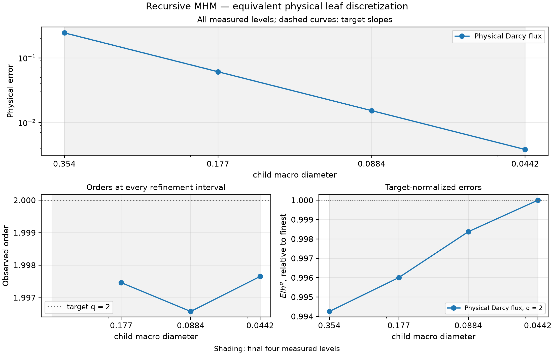
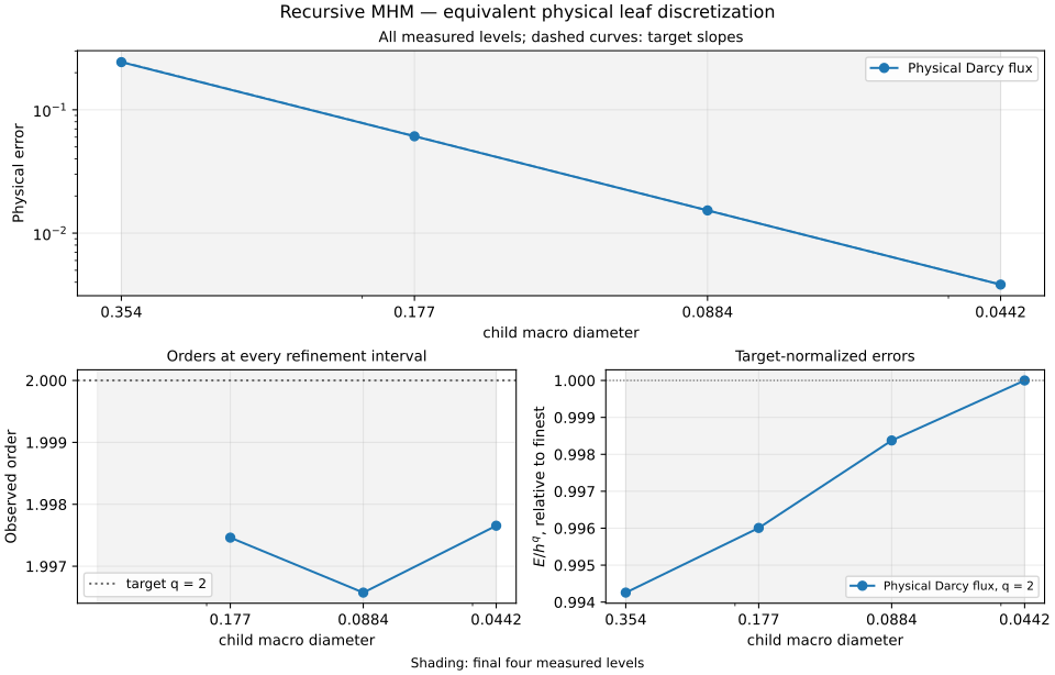
The three consecutive physical-flux orders are 1.99746, 1.99657 and 1.99765; the normalized \(E/H_c^2\) max/min ratio is 1.00578. The physical errors use independent orders 12 and 16 quadrature. Refinement keeps the parent/child/local ratios and degrees fixed. The baseline classical P3 Galerkin calculation in the shared notebook verifies its own refinement on three finer global meshes against the same analytical fields.

PDF · SVG

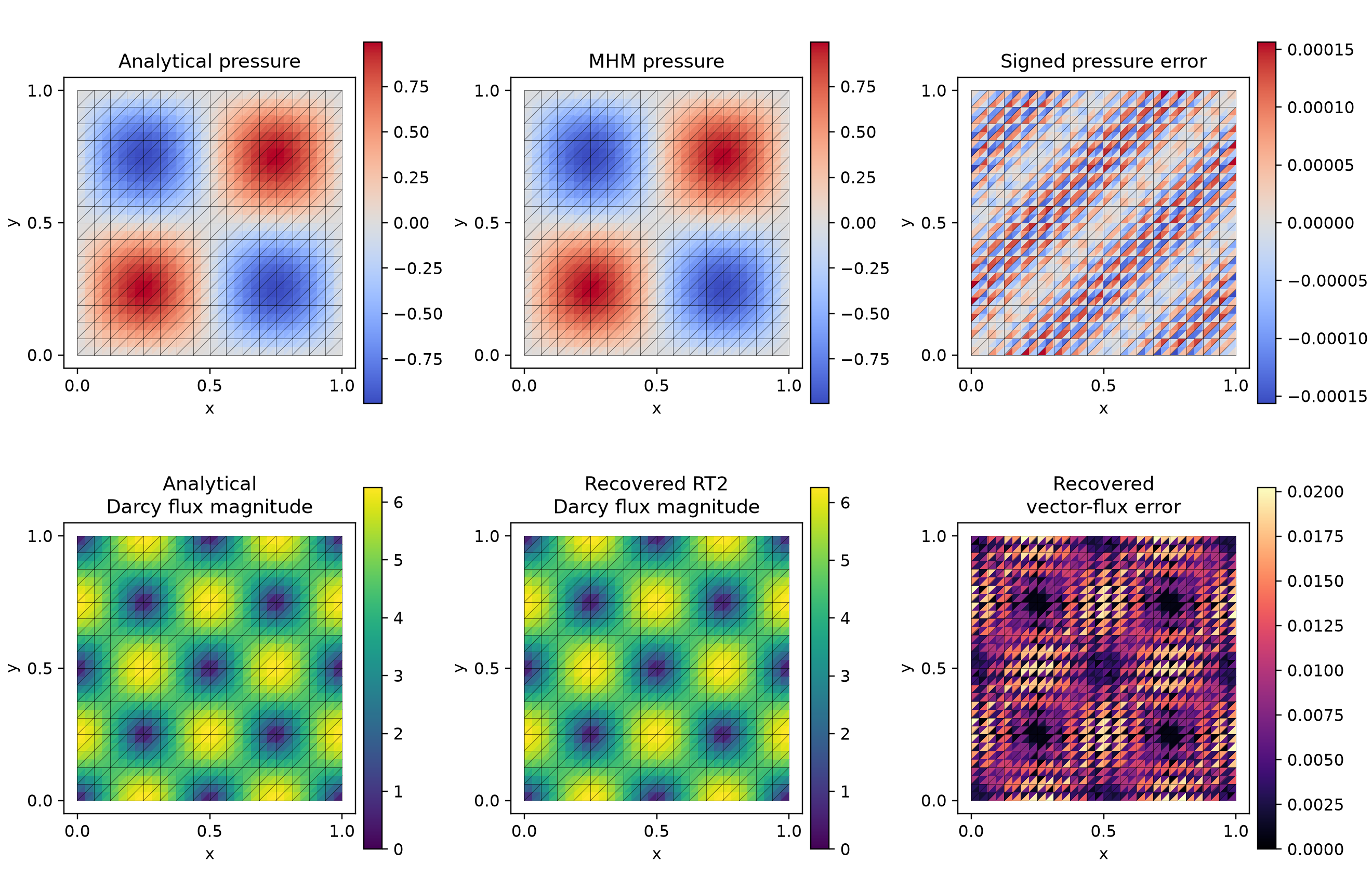
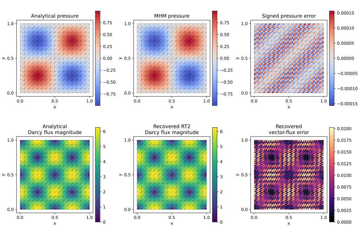
These field panels show the equivalent flattened leaf solution. Equality of its coefficient vectors with the recursive leaves is verified in the table; the illustration corresponds to outer \(n=8\) and 512 child macrotriangles. Each panel overlays that child macro partition, which includes the outer macro edges, and preserves independent fine-cell centroid samples. The flux panels show the RT2 recovery of this same leaf solution; their vector error is distinct from the raw-flux error in the convergence table.

Reproduce this tutorial

The notebook linked at the top defines the forms and runs the recovery, indicator, adaptive and recursive studies. Install the native notebook backend as described in the installation guide, then open it from the source checkout:

pixi run --locked -e introduction jupyter lab notebooks/darcy/reconstruction_and_indicators.ipynb

References

• Christopher Harder and Frédéric Valentin (2016). Foundations of the MHM Method, in Building Bridges: Connections and Challenges in Modern Approaches to Numerical Partial Differential Equations, Lecture Notes in Computational Science and Engineering 114. DOI: 10.1007/978-3-319-41640-3_13.
• Christopher Harder, Diego Paredes and Frédéric Valentin (2013). A family of Multiscale Hybrid-Mixed finite element methods for the Darcy equation with rough coefficients. DOI: 10.1016/j.jcp.2013.03.019.
• Gabriel R. Barrenechea, Larissa Martins, Weslley Pereira, and Frédéric Valentin (2026). An H(div; Ω)-Conforming Flux Reconstruction for the Multiscale Hybrid-Mixed Method, Multiscale Modeling & Simulation 24(2), 399–428. DOI: 10.1137/24M1673073.