Helmholtz MHM

Write a complex plane wave through real and imaginary components, define its outgoing physical data and local/global weak forms, then assemble, solve and postprocess. The refinement figure uses this same declared family.

Complete executable notebook · Download notebook

Run the locked introduction environment. The native UFL path executes; complex coordinates are never discarded. The notebook also preserves a low-frequency affine reproduction control after the plane-wave workflow.

1. Derive the physical operator and boundary data

On the unit square, choose unit density and modulus, \(\omega=10\pi\), \(d=(\cos(\pi/13),\sin(\pi/13))\) and \(p_*(x)=\exp(i\omega d\cdot x)\). Since \(\lVert d\rVert=1\), the independently manufactured volume source is zero:

\[ \begin{aligned} -\Delta p-\omega^2p&=0,\\ \partial_np-i\omega p&=g, &g&=i\omega(d\cdot n-1)p_* \quad\text{on }\partial\Omega. \end{aligned} \]

The unknown interior multiplier is \(\lambda_K=-\partial_{n_K}p\). On the physical exterior, the local impedance and prescribed \(g\) already supply the boundary condition. Exterior multiplier coordinates are fixed zero placeholders; the actual physical exterior flux need not vanish.

Represent pressure by \(z=(\Re p,\Im p)\) with interleaved real coordinates. These are complex coordinates rather than a physical vector. The outgoing term \(-i\omega p\) becomes \(\omega(z_1v_0-z_0v_1)\) in the real weak form.

2. Declare local and global variational equations

The local volume/Robin form and trial/test interface pairings are

\[ \begin{aligned} a_K(p,v)&=(\nabla p,\nabla v)_K-\omega^2(p,v)_K -\langle i\omega p,v\rangle_{\partial K\cap\partial\Omega},\\ b_K(\lambda,v)&=\langle\lambda,v\rangle_{\partial K\setminus\partial\Omega},\\ c_K(p,\mu)&=-\langle p,\mu\rangle_{\partial K\setminus\partial\Omega}. \end{aligned} \]

The notebook first writes wave_forms explicitly. Here exterior is its UFL indicator of the physical boundary, \(x=0,1\) or \(y=0,1\):

z, v = ufl.TrialFunction(V), ufl.TestFunction(V)
x = ufl.SpatialCoordinate(domain)
n = ufl.FacetNormal(domain)
phase = omega*(d[0]*x[0]+d[1]*x[1])
normal_factor = omega*(ufl.dot(ufl.as_vector(d),n)-1)
g = ufl.as_vector((-normal_factor*ufl.sin(phase),
                   normal_factor*ufl.cos(phase)))
a = (ufl.inner(ufl.grad(z),ufl.grad(v))-omega**2*ufl.inner(z,v))*dx
a += omega*(z[1]*v[0]-z[0]*v[1])*exterior*ds
L = ufl.inner(g,v)*exterior*ds

Choose a Basix Q4 element with two real coordinates, on a \(2\times2\) fine subdivision of each macro square. Declare the named field and pairings:

def wave_local(local):
    native = local.native_space(wave_element)
    z,v = ufl.TrialFunction(native.space),ufl.TestFunction(native.space)
    a,L,exterior = wave_forms(native.space,native.mesh)
    b = local.trace_pairings(
        lambda phi,ds: ufl.inner(phi,v)*(1-exterior)*ds,
    )
    c = local.trace_pairings(
        lambda phi,ds: -ufl.inner(phi,z)*(1-exterior)*ds,axis="rows",
    )
    local.field("pressure",native)
    return local.equations(a=a,L=L,b=b,c=c)

The native binding owns coefficient ordering and the interface owns geometric incidence signs. The mathematical signs stay visible in these expressions. No retained static mode is inserted: the selected local wave operators are invertible. Positive frequency alone does not exclude other local resonances.

3. Define meshes, assemble and solve

Use a \(12\times12\) square macro grid with polynomial P2 complex normal traces:

macro = CartesianMacroMesh(12)
skeleton = SkeletonSpace(
    macro,tuple(FaceSpace.uniform(2) for _ in macro.faces),components=2,
)
hierarchy = MeshHierarchy(
    macro,tuple(macro.submesh(i,2) for i in range(len(macro.cells))),
)
interface = bind_interface(skeleton,convention="normal")
problem = bind_problem(
    hierarchy,interface,wave_local,global_equation=Equation(0,0),
)
system = assemble(problem)
fixed = {int(dof):0.0 for face in macro.boundary_faces
                     for dof in skeleton.dofs(int(face))}
solution = solve(system,fixed=fixed)
pressure = solution.field("pressure")

The global equation imposes zero incident pressure jumps on interior faces, with the sign of \(c_K\). The Robin data are already part of each local load. There is no exterior Dirichlet pressure condition or pressure gauge here.

Integrating the physical errors with independent product Gauss rules of orders 10 and 14 gives relative pressure error \(1.03918\times10^{-3}\) and relative broken gradient error \(5.07579\times10^{-3}\). These native norms agree with the attributed convergence record's n12 observations to about \(4.3\times10^{-11}\) relatively. A separate original uncondensed coefficient-row check is accepted with relative residual \(3.55\times10^{-14}\); it does not replace the physical error integration.

4. Independently refine the classical reference

Assemble the same wave_forms on a single conforming global Q4 mesh, with the same outgoing data, through MultiscaleProblem.from_global. This reference uses no local response elimination or MHM multiplier. The native space is closed explicitly; its portable coefficient map retains the declared nodal basis for subsequent evaluation.

Global subdivisions	Relative pressure \(L^2\)	Relative broken gradient \(L^2\)
16	\(3.9855\times10^{-4}\)	\(2.4560\times10^{-3}\)
32	\(1.2523\times10^{-5}\)	\(1.5763\times10^{-4}\)
64	\(3.9272\times10^{-7}\)	\(9.9183\times10^{-6}\)

Both analytical norms decrease on the refined global grids. The finest reference is substantially more accurate than the coarse MHM illustration; it remains a numerical approximation. Its global compatibility residual stays below \(2.2\times10^{-16}\).

5. Plot the wave, reference and physical errors

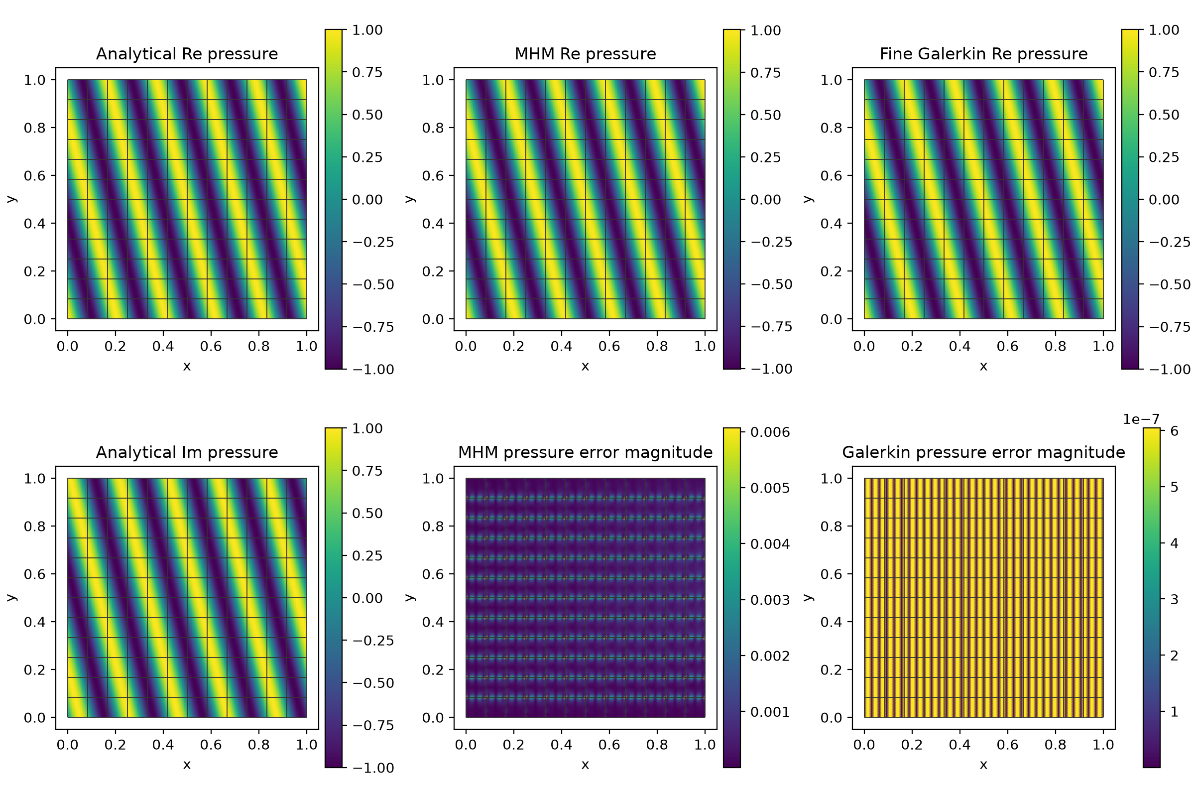
Analytical, MHM and refined conforming wave fields and complex pressure errors

Every panel highlights the actual square macro mesh. Macrocells retain independent one-sided pressure values. Independent colorbars expose the reference's much smaller complex pressure error without merging scales.

6. Reach the fixed-frequency asymptotic regime

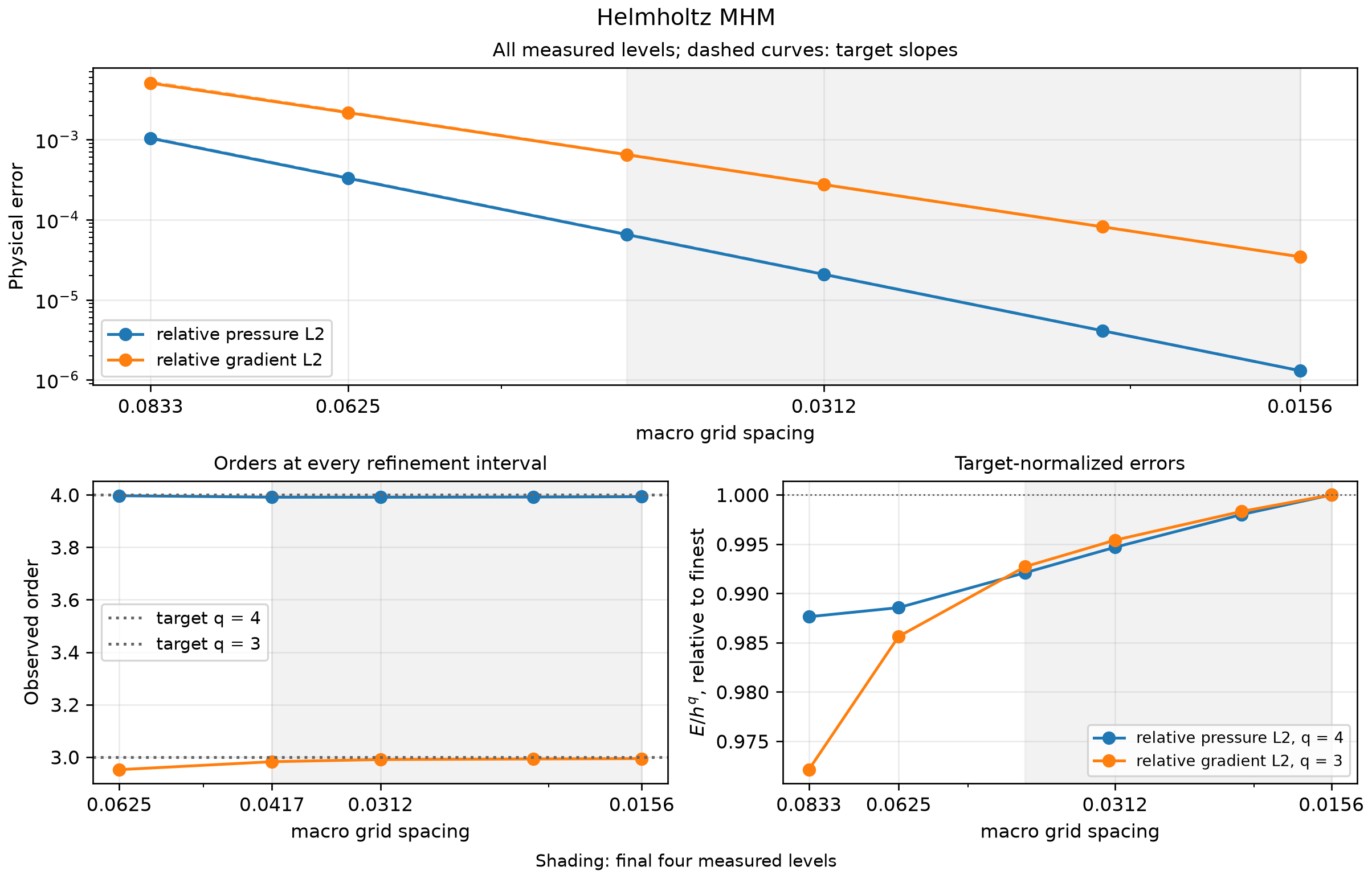
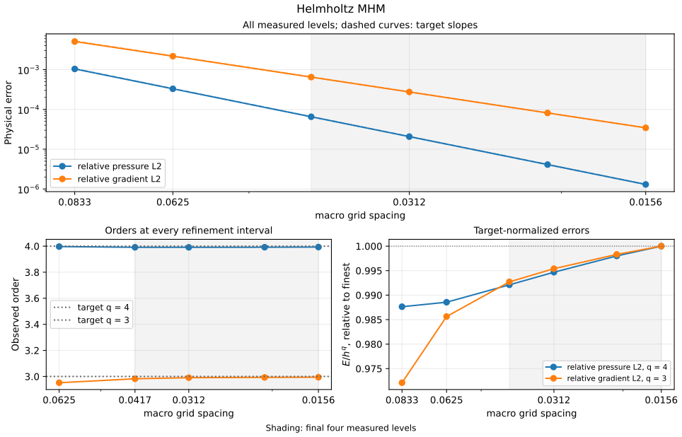
The smooth fixed-frequency study uses polynomial trace degree two and local Q4 pressure on refined Cartesian cells. It targets pressure order four and gradient order three after the frequency and local error are resolved. The recorded errors are PyMHM observations against the analytical field, not values digitized from a paper. This analytical variant is distinct from a matched reproduction of the published curves.

Physical errors and successive observed rates

Vector SVG · Publication PDF

Observable	Expected order	Last three orders	Maximum/minimum of \(E/H^q\)
relative pressure \(L^2\)	4	3.9910, 3.9918, 3.9930	1.0080
relative gradient \(L^2\)	3	2.9906, 2.9928, 2.9941	1.0073

The plotted sequence retains all six measured levels. Its final four levels are \(n=24,32,48,64\). The refinement variable is the square edge length; non-dyadic consecutive rates use the actual grid-spacing ratios. Normalized amplitudes vary by less than one percent across this window. The comparison concerns fixed frequency, smooth analytical data and resolved local polynomial approximation. It does not give a frequency-uniform pollution bound or transfer these rates to resonant or unresolved heterogeneous data. The polynomial one-level estimate is Theorem 5.4 of Chaumont-Frelet and Valentin (2020): it additionally requires sufficiently small \(\omega H\) and \(C_s(\omega)(\omega H)^{\ell+1}\), global uniqueness, and a regular macro mesh compatible with the piecewise smooth coefficient partition. It omits local finite element error; the Q4 local discretization above is a separate approximation whose accuracy must be resolved.

Numerical record, SHA-256 fcfae8fd22ded4b560dc6ad6fbfb7aecca7da8e2a5681cffaeff886ea6d12e9e.

References

Théophile Chaumont-Frelet and Frédéric Valentin (2020). A Multiscale Hybrid-Mixed Method for the Helmholtz Equation in Heterogeneous Domains. SIAM Journal on Numerical Analysis 58(2), 1029–1067. DOI: 10.1137/19M1255616.