Mapped hexahedral RT flow around a well

solve_darcy_mapped_rt provides a three-dimensional mixed MHM formulation on conforming trilinear hexahedra. It uses tensor-product Raviart–Thomas fluxes, local discontinuous pressure and oriented normal-flux moments on quadrilateral macrofaces. The RT1 configuration is the hexahedral family used in Durán et al. (2019), §7.4. This is an H(div) formulation in three dimensions; it is distinct from a tetrahedral primal pressure approximation.

Mapping, spaces and physical equations

Let \(F_K:[0,1]^3\to K\) be a trilinear map, with Jacobian \(J\). The flux and its divergence satisfy the contravariant Piola identities

\[ q(F_K(\widehat x))=\frac{J\widehat q}{\det J},\qquad \operatorname{div}q(F_K(\widehat x))= \frac{\widehat{\operatorname{div}}\widehat q}{\det J}. \]

For RT1, the reference vector space is \(Q_{2,1,1}\times Q_{1,2,1}\times Q_{1,1,2}\), and pressure is the ordinary scalar pullback of \(Q_{1,1,1}\). Each oriented face has four integral Legendre normal moments. On a genuinely nonaffine cell, the divergence belongs to \(Q_1/\det J\); it does not generally lie in the scalar-pullback pressure space. The discrete equations enforce all pressure-tested divergence/source moments, including the constant test giving fine-cell mass conservation.

A HexSkeleton prescribes a piecewise tensor-polynomial reference-face flux density. Its pullback corresponds to a physical normal density divided by the surface Jacobian. Subfaces must align with the local reference grid, and their degree must not exceed the local RT degree. The implementation preserves face orientations and tensor-coordinate permutations. When the skeleton resolves every fine normal trace, local condensation yields the classical globally conforming mixed discretization; changing macro grouping then leaves the physical fields unchanged.

The constitutive equation is \(K^{-1}q+\nabla p=0\). Permeability may be a positive scalar, SPD tensor, or physical-coordinate callback. Heterogeneous interfaces must be resolved by the cells/integration. Dirichlet pressure is weak data; Neumann input is the physical outward normal flux. A pure Neumann problem uses the physical integral of pressure as its gauge. Local flux and pressure units are balanced by an exact symmetric change of coordinates, and physical fields are restored before error or conservation measurements. The returned physical_residuals separately checks constitutive, divergence and prescribed normal-moment equations through a blockwise backward-error criterion.

HexMesh checks tensor connectivity, opposite outward orientations and positive sampled Jacobians. The latter is not a proof of global injectivity for arbitrary warped input meshes. The present geometry maps have straight-edged polygonal faces; exact cylindrical or general CAD surfaces are a separate capability.

Dupuit–Thiem data and declared reservoir geometry

The analytical case uses the physical parameters in Durán et al. (2019), Table 1:

Quantity	Value
Reservoir height \(H\)	10 m
Well / exterior radius	0.2 / 50 m
Permeability \(\kappa\)	\(10^{-13}\) m²
Viscosity \(\eta\)	0.001 Pa·s
Exterior pressure \(p_e\)	25 MPa
Rate parameter \(Q\)	0.01 m³/s

The exact pressure and Darcy flux are

\[ p=p_e+\frac{Q\eta}{2\pi\kappa H}\log(r/r_e),\qquad q=-\frac{Q}{2\pi H}\frac{(x,y,0)}{r^2}. \]

Here positive \(Q\) denotes production: pressure is lower at the well, the outward rate through the inner boundary is \(+Q\), and the exterior rate is \(-Q\). This follows directly from \(q=-(\kappa/\eta)\nabla p\) and agrees with the pressure trend in Figure 14. The printed analytical expression has the opposite sign for the positive rate listed in Table 1; the physical convention used here is explicit.

As in §7.4, analytical pressure is imposed on both the inner and outer lateral boundaries, while the top and bottom are impermeable. The rate is a parameter of the analytical Dirichlet data, rather than a separately imposed Neumann condition. On the polygonal boundary, the exact pressure is evaluated at the actual physical position; it is not replaced by a circular-boundary constant.

The macro grid has eight azimuthal sectors and four radial bands, giving 32 hexahedra. The five declared radii are approximately \(0.2,0.795270729,3.162277660,12.574334297,50\) m. These logarithmically spaced radii define an original explicit geometry. The paper's printed graded-distance expression \(2^{-m}r_w\), \(m=1,\dots,5\), does not determine radii spanning its stated domain. Figure 12 establishes the topology but not unique numerical radii, so identical historical geometry is not asserted.

Fixed fine grid and macro refinement

The four macro factors are 1, 2, 4 and 8, with local refinements 8, 4, 2 and 1. Thus all four runs share 16,384 fine hexahedra. The last is the classical mixed RT1 limit. This follows the scale relation of §7.4 while retaining the explicit radial geometry above. A second study refines the classical RT1 grid through five fine factors, 1, 2, 3, 4 and 8. Physical volume norms, quadrature checks, integrated boundary rates and source/flux balances are recorded for each run.

Macro cells	Trace + coarse unknowns before boundary elimination	Relative pressure-increment error	Relative flux error
32	576	0.37456%	2.02284%
256	3,968	0.18077%	0.44303%
2,048	29,184	0.17828%	0.13043%
16,384	223,232	0.17824%	0.06345%

The independently refined classical grids have flux errors of 4.7694%, 1.0174%, 0.4522%, 0.2541% and 0.06345%. At the finest level, the integrated extraction rate is 0.009999995731 m³/s, compared with the exact 0.01 m³/s. The maximum fine-cell pressure-tested divergence moment is below \(5.0\times10^{-16}\). The pressure error at fixed fine resolution approaches a local-discretization floor; further macro refinement primarily improves the flux in this study.

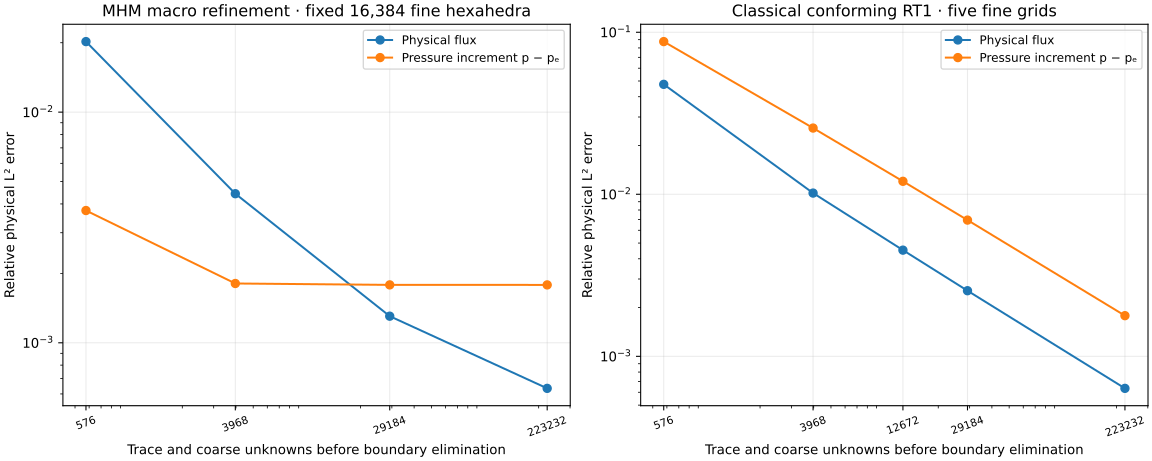
Pressure-increment errors are normalized by \(\|p-p_e\|_{L^2}\), and flux errors by \(\|q\|_{L^2}\). Records also contain absolute norms and the error normalized by \(\|p\|_{L^2}\); the latter can look small because of the 25 MPa background. The original units are retained throughout.

The spatial panels and profiles use the declared geometry, physical data, RT1/Q1 spaces and quadrature orders. The field replay receipt identifies their coefficient and source digests and independently integrated physical norms and boundary rates. Each field is evaluated from its own archived fine-cell connectivity and coefficients with the canonical tensor-product RT1 basis and Piola mapping. The finest plotted field has a maximum pressure-tested divergence moment of \(6.57\times10^{-16}\) m³/s, or \(6.57\times10^{-14}\) relative to the prescribed rate. Its maximum physical block backward residual is \(1.71\times10^{-11}\), below the unchanged \(10^{-10}\) acceptance criterion. The replay record distinguishes these field diagnostics from the convergence acquisition.

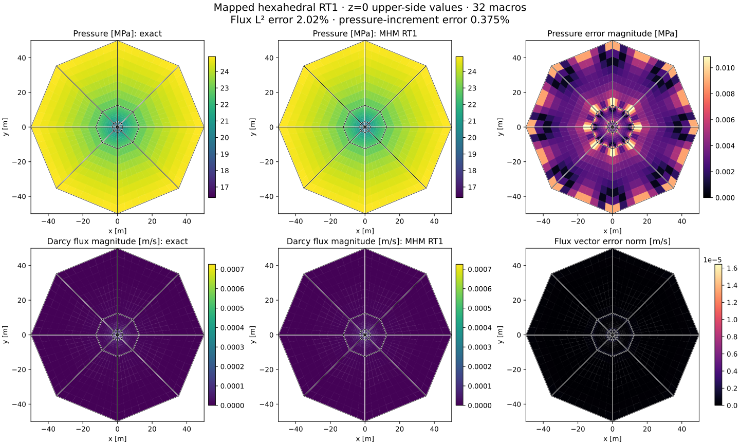
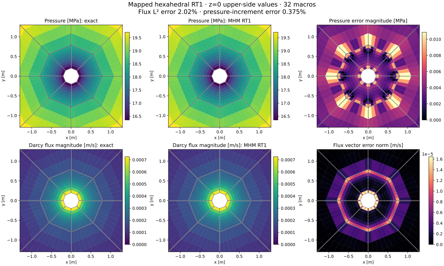
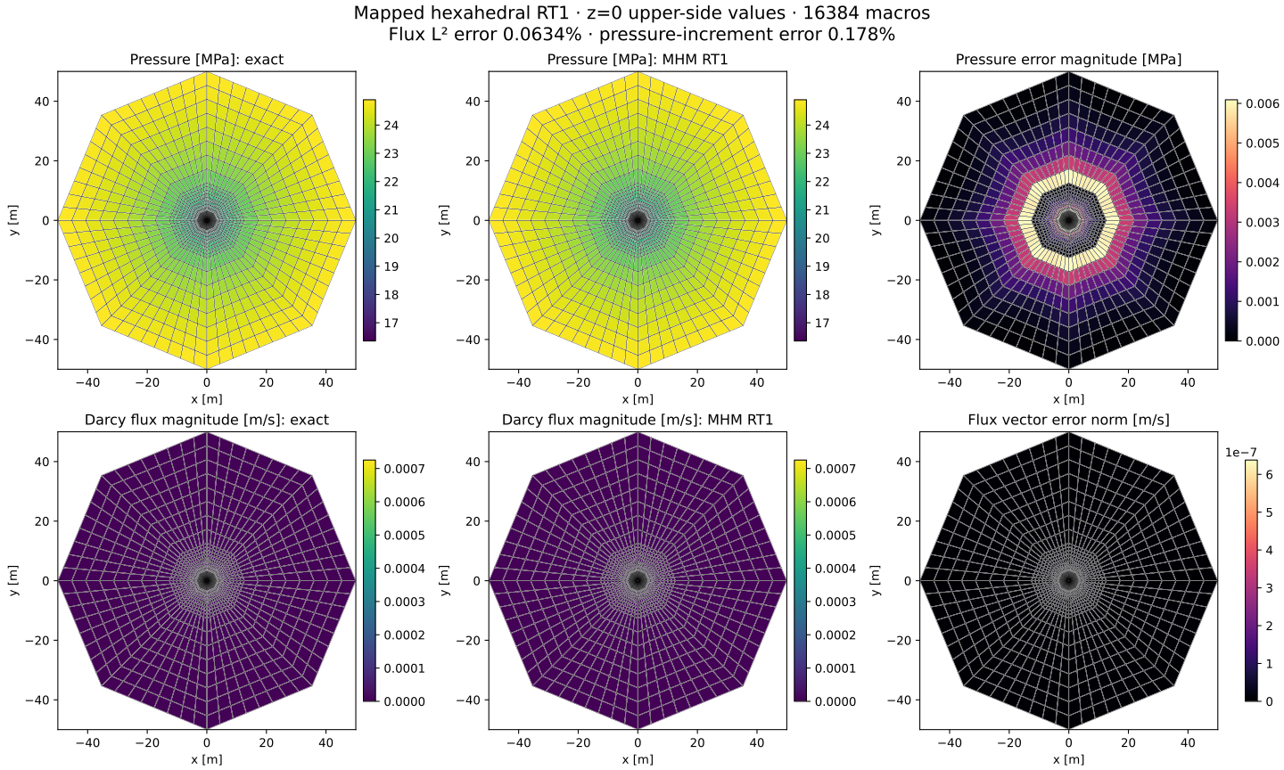
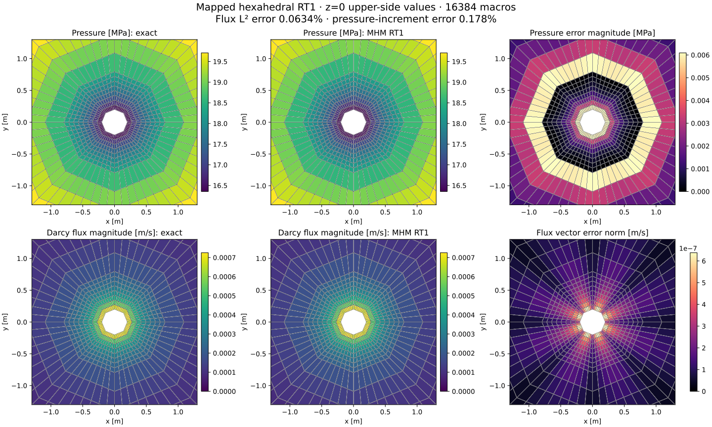
The plots use the upper incident cells at \(z=0\), with independent fine-cell centroid samples and the actual macro intersections. Pressure and flux are not smoothed across interfaces. Exact/numerical panels share scales; the final column shows the scalar pressure error or the norm of the vector flux difference. The physical L2 errors are integrated over volumes, independently of the display samples.

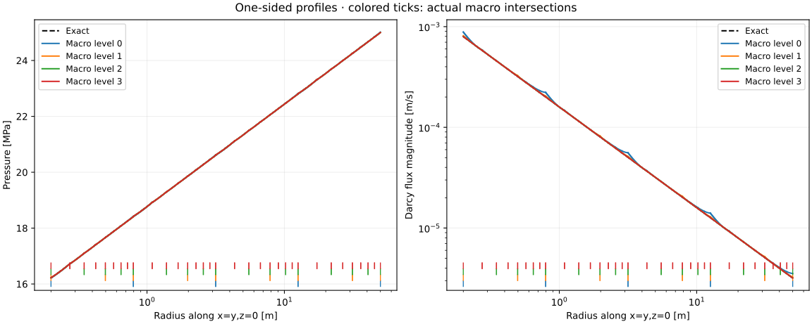
The profiles follow \(x=y,z=0\) from the incident azimuthal sector below \(\pi/4\). Fine intervals are drawn separately, and colored ticks identify actual radial macro boundaries. This preserves one-sided pressure and tangential flux values instead of averaging along a macroface.

Verification and reproducibility

The core tests verify Piola divergence by Cartesian differentiation, canonical normal moments, the divergence theorem, shared-face rotations, sources, Dirichlet/Neumann signs, pressure gauges, physical-unit invariance and equivalence of fully resolved macro partitions. Independent DOLFINx/UFL tests compare complete RT0, RT1 and RT2 mixed matrices and loads on a nonaffine hexahedron with a variable anisotropic tensor. These establish operator consistency; they do not replace mesh refinement or prove parameter-independent stability on arbitrary maps.

The original acquisition and replay drivers are examples/solve_mapped_well.py and examples/plot_mapped_well.py. Numerical fields, physical diagnostics and source/field digests are archived in examples/results/mapped-well/. Notebook 44_mapped_well.ipynb displays the recorded studies. The oscillatory three-dimensional coefficient of Problem 5 in Durán et al. (2019) and its historical field profiles are not part of this analytical campaign.

The global retained saddle can be resolved with an explicit global_rtol and global_refinement_precision="extended". Defaults preserve double-precision behavior. Extended correction accumulation requires a wider long-double type; the physical mixed-block acceptance criterion remains unchanged. A stricter linear-solver target is a numerical accuracy request, not a guarantee of an attainable physical residual for every parameter scale.

References

• Omar Durán, Philippe R. B. Devloo, Sônia M. Gomes, and Frédéric Valentin (2019). A multiscale hybrid method for Darcy’s problems using mixed finite element local solvers, Computer Methods in Applied Mechanics and Engineering 354, 213–244. DOI: 10.1016/j.cma.2019.05.013.