Quarter-five spot: point wells and a low-permeability obstacle

The quarter-five-spot experiments have injection at (1,1), extraction at (0,0), impermeable exterior boundaries and a zero domain-mean pressure. With \(q=-K\nabla p\), injection has a positive source and extraction a negative source. Pressure is higher near injection, and flux connects the two wells while respecting material barriers.

The published point-well problem

Harder, Paredes and Valentin (2013), §5.2, consider both K=1 and layered permeability. The lower layer has K=1000 and the upper layer K=1, with interfaces at y=0.5 and y=0.484375.

Araya et al. (2013), §6.3, explicitly model the wells by Dirac loads and note the example's singular regularity. The numerical functional used here is

\[ f(v)=v(1,1)-v(0,0). \]

The unit intensity is an explicit normalization: the published discussion does not provide a recoverable well rate. Each point load is shared between incident macrocells in proportion to their actual angles. The weights sum to one, preserving the prescribed total well rate. Primal Pk applies the exact discrete point functional; the mixed P0 test space receives the integrated well rate in incident fine cells. No finite-area source is substituted in this point-well experiment.

The homogeneous Neumann data describe the exterior edges away from the corner well points; the signed corner functional supplies their rates in the discrete weak problem. Zero boundary trace coefficients impose those Neumann data. For primal P2 this is a weak boundary convention, and the raw gradient flux can have nonzero pointwise exterior normal values. The mixed RT0 field instead satisfies the prescribed fine-edge normal moments exactly, up to solver error.

The comparison uses 32×32 squares split along the southwest-to-northeast diagonal, 2048 macrotriangles, two local subdivisions and constant traces. Primal pressure is P2; the mixed method is RT0/P0. The offset material interface cuts macrotriangles but aligns with the fine mesh. The paper specifies its resolution but not enough connectivity details to assert identical historical matrices.

Independent assembly of the six discrete cases

An independently assembled Basix reference executes all three materials in both local spaces, with the same 2048 macrotriangles, 8192 fine triangles, point allocations, exterior data and physical zero-mean pressure. It solves the original uncondensed saddle system: 33,729 unknowns for primal P2 and 41,921 for mixed RT0/P0. The reference uses FEniCS Basix 0.9.0, basix.finite_element, revision 19555f5b for its executed polynomial and Piola bases, together with SciPy SuperLU. This is an instrumented independent comparison, not an original-author application.

Pressure, raw gradient and physical Darcy flux are compared in broken physical L2 norms on the common fine partition, with independent one-sided values and the native norm as denominator. A positive four-point Gauss rule in each coordinate of a triangle Duffy map integrates these polynomial squared norms exactly up to floating-point arithmetic. Across the three P2 cases, the largest relative differences are 3.02×10⁻¹¹ in pressure, 1.43×10⁻¹¹ in raw gradient and 1.71×10⁻¹¹ in Darcy flux. Across the three RT0/P0 cases, they are 7.30×10⁻¹⁵ in pressure and 7.27×10⁻¹² in Darcy flux.

The reference evaluates the original physical equations separately from its gauge equation; their relative load residual is at most 8.87×10⁻¹³. Inserting the PyMHM fields into the independently assembled physical equations gives at most 1.35×10⁻¹¹. The reference uniformly uses extended residual and coefficient accumulation with the fixed double-precision operator. A further correction of those same equations changes its physical fields by at most 1.13×10⁻¹⁵ relatively. Replay from the archived executed bases is identical with one and two native threads. The verification record identifies the sources, bases, maps, inputs and coefficients. This establishes discrete agreement for the specified cases; it does not establish continuum accuracy or recover the historical well intensity and connectivity.

Expected result. Pressure has logarithmic corner singularities and flux grows near both wells. Their peak values depend on mesh resolution and display sampling; equal peak values on different meshes are not an accuracy criterion. For homogeneous permeability, pressure is antisymmetric under a half-turn about the center. Flux is directed from injection toward extraction.

The red line is the material interface; dark edges are the macro mesh. The high-permeability lower layer carries substantial flux with a comparatively small pressure gradient. The offset case exercises transmission inside macrocells. Broken fields are retained on both sides of every interface.

The local-solver comparison in Figure 19

Figure 19 in §5.2.2 specifically uses the offset interface at \(y=0.484375\), constant skeletal traces \(\ell=0\), and a structured macro mesh with 32 triangles along each domain side. Each macrotriangle has two subdivisions along each edge. The local pressure space is continuous P2 in the primal method; the mixed local method uses the lowest-order Raviart–Thomas element. Its plotted quantity is the magnitude of the physical Darcy flux, denoted \(\sigma(p_h)\) in the article. The primal flux is evaluated as \(-K\nabla p_h\); the mixed method approximates the flux directly in RT0.

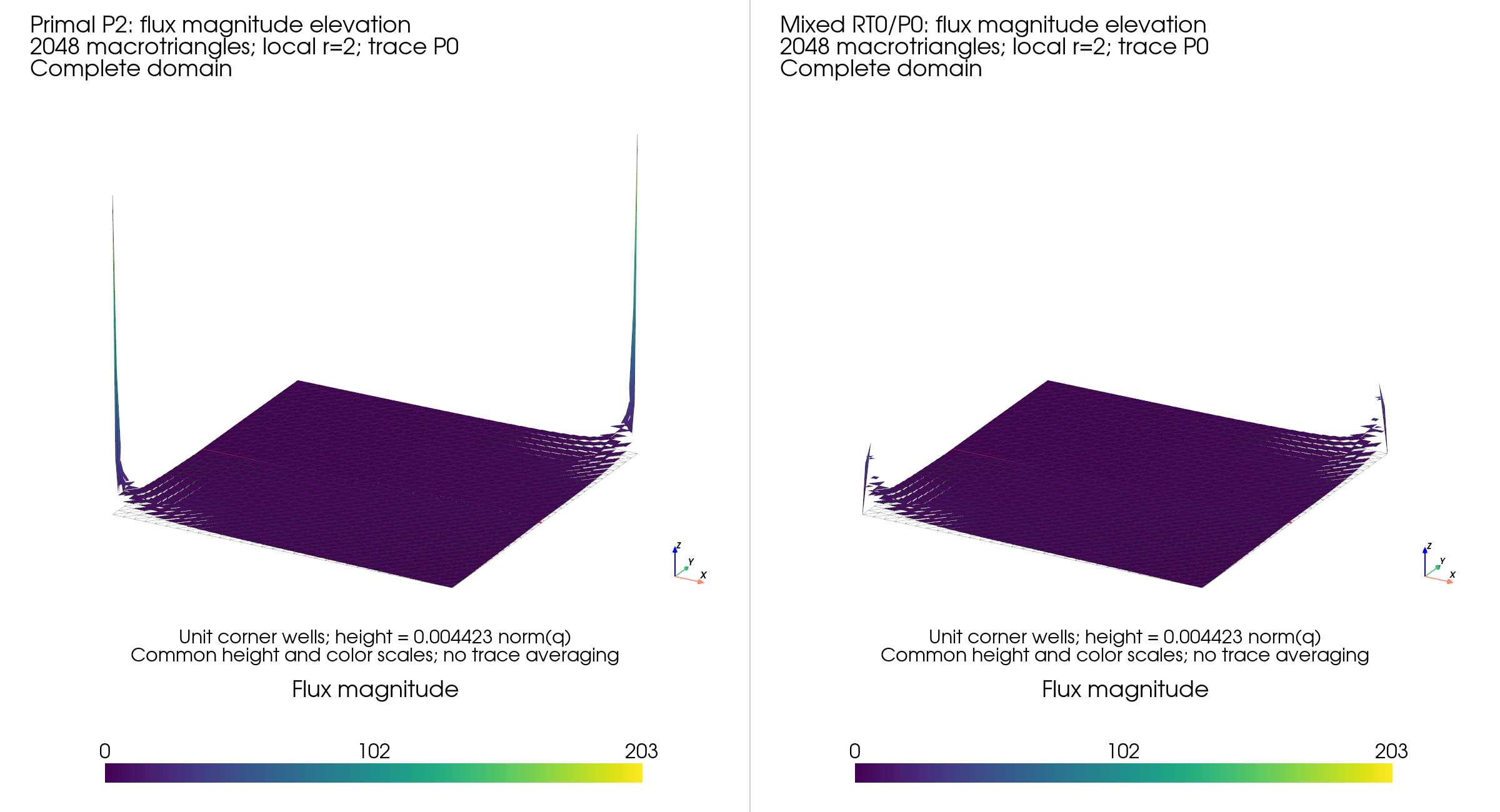
The corresponding PyMHM fields use the stated local spaces, refinement and interface position, with 32×32 squares split along a fixed diagonal. The point functional has unit injection and extraction rates. The article does not specify a recoverable rate, the discrete allocation of the corner loads, the exact macro connectivity, or the evaluation and interpolation used for Figure 19. These are material qualifications near singular wells: a peak read from a colorbar is not an integrated flux or a convergence measure. The elevation views retain the calculated magnitudes without amplitude rescaling. The recorded one-sided fields retain both sides of the material interface.

The full elevation view uses one common color range, 0–203.459, and a common vertical scale for both methods. The nodal display peaks are 203.459 for P2 and 45.2838 for RT0. The detail view excludes each display triangle intersecting the open disk of radius 0.125 around either well; it uses a common range of approximately 0–6.004 to expose the interface. Only the displayed geometry is restricted: the solutions, well rates and conservation calculations are unchanged. Within each image, both panels use the same camera and height scale. The view metadata records the sampling, excluded radius and physical color limits.

The article reports small localized oscillations near the interface for primal local solves and a conforming H(div) flux for mixed local solves. This distinguishes raw primal flux from RT0 normal-flux conformity; pointwise agreement of their peaks is not expected merely from matching the skeletal degree.

Six refinements against an independent Green series

For K=1, separation of variables gives the zero-mean pressure

\[ p(x,y)=y-\tfrac12+\sum_{m=1}^{\infty} \frac{2\cos(m\pi x)}{m\pi\sinh(m\pi)} \left[(-1)^m\cosh(m\pi y)-\cosh(m\pi(1-y))\right]. \]

Differentiating gives the physical flux. Evaluation uses exponentially scaled ratios and checks 2048 against 4096 terms. The comparison excludes balls of radius 0.125 around both wells and measures area-weighted centroid RMS differences. These are sampled diagnostics, not quadrature-certified L2 norms.

A two-dimensional Dirac source does not define a finite H1-energy pressure solution. Consequently this experiment makes no finite-energy convergence or L2-divergence claim at the wells. Macro conservation includes their exact integrated rates, and the RT0 fine-cell balance includes the allocated rates.

From 128 to 4608 macrotriangles, sampled pressure RMS decreases from 0.01124 to 0.0003692, and flux RMS from 0.3511 to 0.06424. At the finest level, doubling the series changes the flux away from wells by at most 8.3×10⁻¹⁰. Macro balance defects stay below 7.6×10⁻¹⁵, and the full original physical-equation residual stays below 3.6×10⁻¹⁴ relative to the point load. Every level retains its executed physical coefficients and evaluation matrices; the six-level record identifies the archives by SHA-256.

Supplemental central obstacle

The square-obstacle quarter-five spot is a separate specified benchmark. In the unit square, define

\[ a=0.25,\qquad b=0.75,\qquad D=[a,b]^2. \]

The obstacle is centered at \((0.5,0.5)\), with side length \(0.5\) and area 0.25, or 25% of the domain. Its permeability is \(10^{-4}\), against a background of 1:

\[ K(x,y)=\begin{cases}10^{-4},&(x,y)\in D,\\1,&(x,y)\notin D,\end{cases} \qquad -\nabla\cdot(K\nabla p)=f,\qquad q=-K\nabla p. \]

Fixed square wells use source −100 on \([0,0.1]^2\) and +100 on \([0.9,1]^2\), hence integrated rates −1 and +1. These finite-area wells remain unchanged during refinement. All exterior normal fluxes are zero, and pressure has mean zero.

Expected result. Most flow bypasses the obstacle through the surrounding permeable region. Pressure gradients can be steep near its corners, but normal flux must balance across interfaces. Concentrated Darcy flux in a thin conductive corridor is physical. Verification includes material integrals, integrated well rates and the linear-system residual.

The cross-code experiment uses 200 macrotriangles from a uniform 10×10 square grid, each split along its southwest-to-northeast diagonal. The obstacle boundary crosses macrocell interiors: 38 macrotriangles contain positive areas of both materials. The well boundaries remain on macrofaces. Local refinement uses four, eight or sixteen subdivisions per macroedge, with one or two constant trace segments; the eight- and sixteen-subdivision meshes also use four segments. These local meshes fit the material interface exactly: their coordinate spacings are 0.025, 0.0125 and 0.00625, respectively. The permeability is constant within each fine triangle, including those inside heterogeneous macrocells. Basix tabulates the P1 basis and quadrature for an independently assembled full primal saddle system, including signed skeletal moments and the physical mean-pressure gauge. NeoPZ supplies the native RT0 operator, with the prescribed boundary fluxes, macro trace restriction and mean gauge applied to that operator. This algebraically restricted reference is distinct from NeoPZ's native MHM controller. Each comparison verifies the original or restricted physical equations before comparing fields.

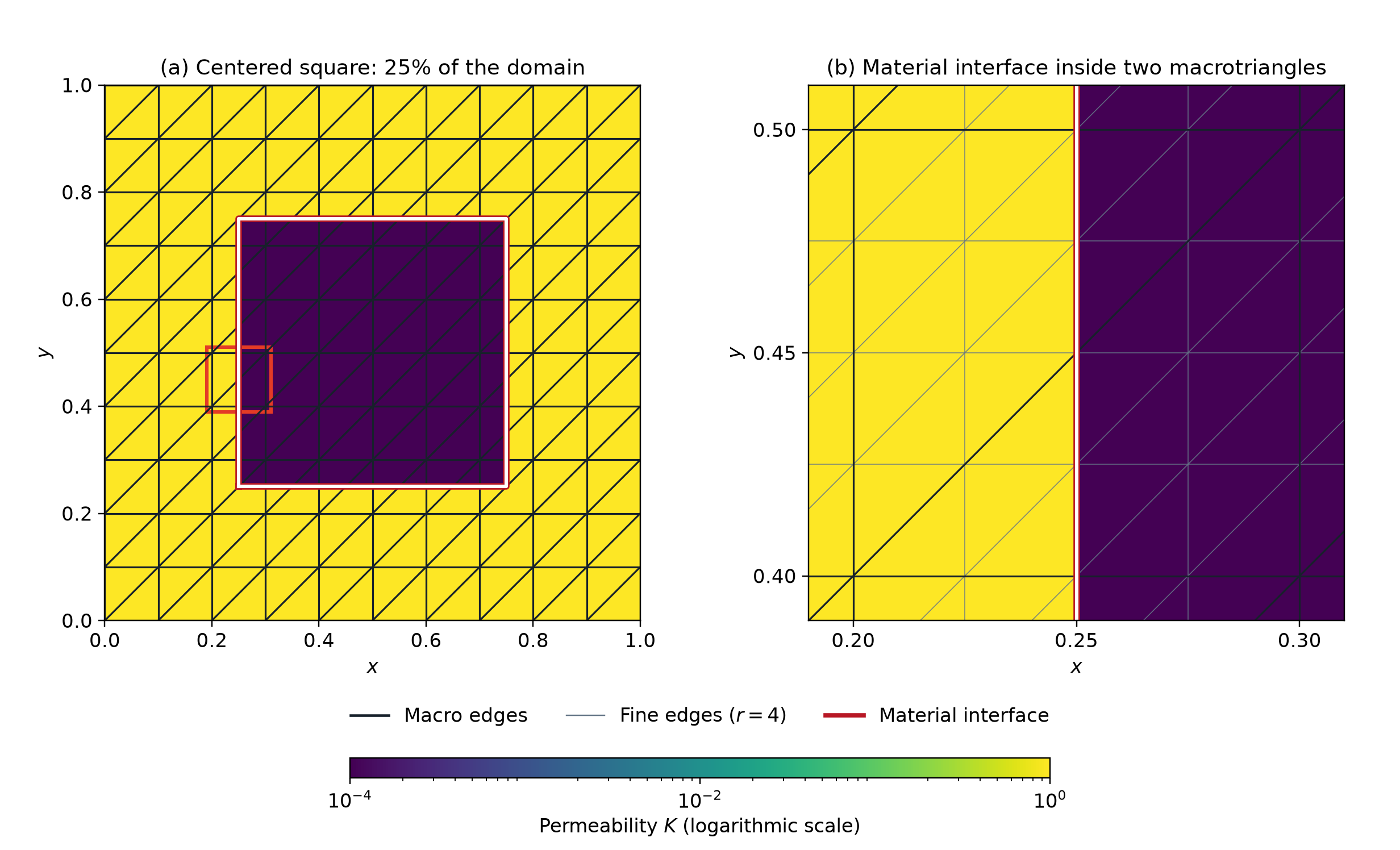
Material interfaces inside macrocells

The local solves retain the two permeability values within each cut macrocell; they do not replace them by one averaged coefficient. The primal method computes a continuous local P1 pressure and its raw flux \(-K\nabla p_h\). That raw flux need not have continuous normal components across fine faces. The mixed local method computes RT0 flux and P0 pressure, with \(\nabla\cdot RT0=P0\). Its normal-flux conformity and fine-cell balance follow from the compatible mixed spaces and the restriction of macroface fluxes to the prescribed skeletal space, as in Durán et al. (2019), §§3.2–3.3. Normal continuity does not require tangential flux continuity across a permeability jump.

Macro, local and skeletal resolution have distinct roles. The obstacle interface crosses macrofaces at their midpoints: a one-segment trace cannot represent separate values on the two material portions, whereas two segments place an endpoint at the intersection. Refining the local solves does not eliminate the approximation imposed by a fixed skeletal space. In particular, Chaumont-Frelet, Paredes and Valentin (2026), §§3–6 derive strengthened estimates on nonaligned macro meshes under the additional assumption that each skeletal subface belongs to one material region. Here the two-segment configuration meets this geometric condition; the one-segment configuration does not. The present comparison verifies matching discrete operators with submacro heterogeneity; it does not claim that convergence result or a computation with material interfaces cutting the fine elements.

Classical mixed reference

A classical global RT0/P0 reference retains independent normal-flux degrees of freedom on all fine faces, including those crossing the macro skeleton. The MHM flux instead belongs to the subspace defined by the one- or two-segment macro trace restrictions. Comparing these spaces on the same material-aligned fine mesh separates the effect of the skeletal restriction from local refinement. Successive classical refinements measure reference sensitivity; this numerical reference is not an exact solution. Both formulations impose zero exterior normal flux and zero mean pressure.

The classical reference uses local-equivalent subdivisions \(r=4,8,16,32\). Its successive relative flux difference is \(\|q_{r}-q_{r/2}\|_{L^2}/\|q_r\|_{L^2}\), with the corresponding definition for pressure. Fields on nested meshes are compared by integration on the finer triangles. The MHM trace study holds \(r=16\) fixed and uses one, two or four segments per macroface. Its same-grid differences use the classical \(r=16\) field norm; the comparisons with \(r=32\) use that finer reference norm. The last classical refinement increment provides a sensitivity scale, not an error bound.

Classical refinement	Fine triangles	Free flux and pressure unknowns	Relative pressure change	Relative flux change
4	3,200	7,920	—	—
8	12,800	31,840	2.06108%	5.30059%
16	51,200	127,680	1.02736%	2.99132%
32	204,800	511,360	0.512606%	1.72552%

The unknown counts exclude exterior fluxes fixed to zero and the additional mean-pressure multiplier. The finest field norms are \(\|p\|_{L^2}=0.7533793\) and \(\|q\|_{L^2}=1.9325449\). NeoPZ supplies the native RT0/P0 matrices and field evaluation; SciPy SuperLU solves the global system with the physical mean-pressure gauge. The three-point positive triangular quadrature integrates the squared RT0 and P0 differences exactly on these nested affine meshes, up to floating-point evaluation and summation. The classical fields satisfy \(\int_\Omega K^{-1}|q_h|^2=\int_\Omega p_h f\) with a relative defect below 4.76×10⁻¹⁶; the relative residual of the original free algebraic equations is at most 8.80×10⁻¹³. The energy identity uses the homogeneous normal-flux boundary condition and the resolved source.

MHM trace segments per macroface, at \(r=16\)	Pressure difference / same-grid classical pressure norm	Flux difference / same-grid classical flux norm
1	26.5680%	42.8987%
2	0.422949%	6.20369%
4	0.0946676%	2.54342%

The two-segment trace resolves the midpoint material intersections; four segments further enrich the same RT0/P0 MHM approximation. The four-segment result is included in the matched NeoPZ comparisons below. Comparing those MHM fields with the finer classical \(r=32\) field gives:

MHM trace segments, at \(r=16\)	Pressure difference / classical \(r=32\) pressure norm	Flux difference / classical \(r=32\) flux norm
1	26.6235%	42.9397%
2	0.689218%	6.44000%
4	0.528682%	3.07375%

The classical flux changes by 1.72552% on its last refinement. Reference sensitivity remains material for the four-segment comparison, which requires further classical refinement before an accuracy claim. These percentages remain differences between numerical fields. They are not certified errors against the exact PDE solution, including when the MHM/classical difference is smaller than that last refinement increment.

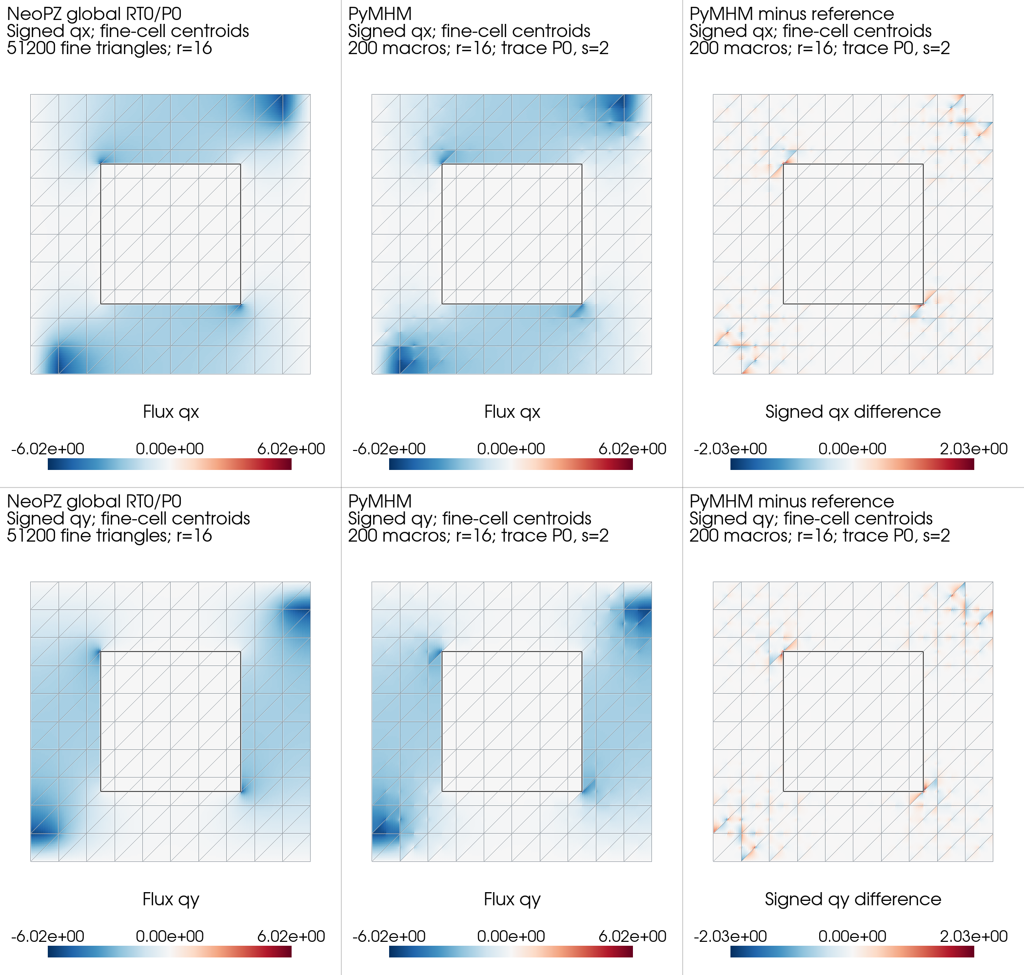
Matched MHM fields

Reference	Matched configurations	Largest pressure L2 difference	Largest flux L2 difference
Basix, independently assembled primal P1	8	1.44×10⁻¹¹	2.77×10⁻¹²
NeoPZ EHDivConstant, restricted RT0/P0	8	7.62×10⁻¹³	2.28×10⁻¹²

The full original Basix saddle residual, normalized by its physical load, is at most 9.61×10⁻¹³. The corresponding gauge-augmented restricted NeoPZ residual is at most 3.30×10⁻¹³. The native RT0 fine-cell balance defect is at most 7.12×10⁻¹⁵. The PyMHM macro balance defect is at most 7.41×10⁻¹⁴; its full original free-equation residual is at most 6.04×10⁻¹¹, with the physical load as denominator. Pressure integrals have magnitude at most 3.38×10⁻¹⁶ and exterior trace values are zero. Basix assembly orders six and eight change the integrated pressure and flux by at most 1.26×10⁻¹¹ and 1.80×10⁻¹², respectively. The material and well interfaces fit the fine mesh, so these integrands are polynomial on every integration cell. These compare matching discrete formulations; agreement between codes does not by itself measure their error against the exact PDE solution.

The component panels display signed \(q_x\) and \(q_y\), with symmetric color scales centered at zero and a shared range for each reference/PyMHM pair. The arrows show the normalized vector \(q/|q|\) at actual fine-cell centroids selected by spatial bins. The same centroids are used for both implementations; their plotted length is fixed at 0.035 in unit-domain coordinates. Arrow length does not encode flux magnitude: the underlying color field supplies the magnitude. No field interpolation or averaging across material interfaces is applied.

Difference panels use their own small color scales; their patterns must be interpreted against the reported absolute values. Flux difference means the norm of the vector difference, not subtraction of the two magnitudes.

The numerical records identify Basix 0.9.0, module basix.finite_element, revision 19555f5b, and NeoPZ, module TPZMixedDarcyFlow with EHDivConstant, revision 4c6b6d27. The upstream sources are unchanged. Private instrumented drivers assemble the comparisons; they are distinct from an original author application. Preserved MSL sources lack a verified upstream revision and executable for this acquisition, so no current MSL execution is attributed. Full revisions, executed basis matrices, coefficient maps, quadrature orders, source fingerprints, gauge conventions and original-equation residuals accompany each archived case.

Reproduction

pixi run --locked -e notebooks python -m examples.plot_quarter_spot
pixi run --locked -e test-core python -m examples.solve_quarter_obstacle --refinements 4 8 16 --segments 1 2 --formulations primal mixed --workers 1 --native-threads 1
pixi run --locked -e notebooks gallery-quarter-elevation
pixi run --locked -e notebooks gallery-quarter-geometry
pixi run --locked -e notebooks gallery-quarter-reference
pixi run --locked -e notebooks gallery-quarter-classical

The source program reproduces the PyMHM point-well cases and analytical-series comparison. --reuse-results redraws archived fields without recomputing them. Reference-program numerical arrays, revisions and measured differences are available in the accompanying records. The obstacle acquisition command runs the original public Darcy solvers; the private independent comparisons are identified by their executed revisions and source digests in the records. The elevation task redraws the offset-layer views. The geometry command displays the material cuts through macrocells and the fitted local mesh. The reference command renders the archived square-obstacle comparisons, including signed components and vector directions, without executing the reference programs. The classical command renders the unrestricted RT0 reference and trace-enrichment study. Notebook 22 checks the geometry and well rates and displays these records.

References

• Christopher Harder, Diego Paredes, and Frédéric Valentin (2013). A family of Multiscale Hybrid-Mixed finite element methods for the Darcy equation with rough coefficients, Journal of Computational Physics 245, 107–130. DOI: 10.1016/j.jcp.2013.03.019.

• Rodolfo Araya, Christopher Harder, Diego Paredes, and Frédéric Valentin (2013). Multiscale Hybrid-Mixed Method, SIAM Journal on Numerical Analysis 51(6), 3505–3531. DOI: 10.1137/120888223.

• Omar Durán, Philippe R. B. Devloo, Sônia M. Gomes, and Frédéric Valentin (2019). A multiscale hybrid method for Darcy’s problems using mixed finite element local solvers, Computer Methods in Applied Mechanics and Engineering 354, 213–244. DOI: 10.1016/j.cma.2019.05.013.

• Théophile Chaumont-Frelet, Diego Paredes, and Frédéric Valentin (2026). Flux approximation on unfitted meshes and application to multiscale hybrid-mixed methods, Computers & Mathematics with Applications 209, 16–27. DOI: 10.1016/j.camwa.2026.01.016.