Oseen MHM

Write a velocity–pressure local problem and its global interface equation with UFL, then assemble, solve and recover the two physical fields. The convection velocity is prescribed; the interface unknown is the half-advection pseudotraction.

Complete executable notebook · Download notebook

Run the notebook in the locked introduction environment. It first verifies an affine Taylor–Hood example, includes independently assembled classical controls, and closes with the separately identified smooth stabilized convergence study.

1. Declare the physical problem

On the unit square, take viscosity and drag equal to one and convection \(\beta=(2,3)\). Choose the solution before assembling any operator:

\[ \begin{aligned} &-\Delta u+(\beta\cdot\nabla)u+u+\nabla p=f,\\ \nabla\cdot u&=0,\\ u_*&=(1-x+2y,-2-x+y),\\ p_*&=x+2y-0.8,\\ f&=u_*+(5,3). \end{aligned} \]

The source follows independently from \(\Delta u_*=0\), \((\beta\cdot\nabla)u_*=(4,1)\) and \(\nabla p_*=(1,2)\). Prescribe the exact velocity on the exterior and the global pressure integral \(0.7\).

def exact_velocity(x):
    return np.column_stack((1-x[:, 0]+2*x[:, 1], -2-x[:, 0]+x[:, 1]))

def exact_pressure(x):
    return x[:, 0]+2*x[:, 1]-0.8

2. Associate meshes and a vector trace

Use Taylor–Hood P2 velocity/P1 pressure on each refined macrotriangle. The vector trace has two components and P1 approximation on each macroface.

macro = TriangleMesh.unit_square(2)
skeleton = SkeletonSpace(
    macro, tuple(FaceSpace.uniform(1) for _ in macro.faces), components=2,
)
hierarchy = MeshHierarchy(
    macro, tuple(macro.submesh(i, 2) for i in range(len(macro.cells))),
)
interface = bind_interface(skeleton, convention="normal")

The binding owns incident normal signs, face numbering and native coefficient maps. These geometric details do not change the mathematical signs below.

3. Write momentum and incompressibility

For divergence-free constant convection, the skew form is

\[ \begin{aligned} a_K((u,p),(v,q))={}&(\nabla u,\nabla v)_K+(u,v)_K\\ &+\tfrac12[(\beta\cdot\nabla u,v)_K-(u,\beta\cdot\nabla v)_K]\\ &-(p,\nabla\cdot v)_K-(q,\nabla\cdot u)_K. \end{aligned} \]

The notebook's oseen_volume_forms contains this form directly:

u, p = ufl.TrialFunctions(W)
v, q = ufl.TestFunctions(W)
x = ufl.SpatialCoordinate(domain)
beta = ufl.as_vector((2.0, 3.0))
truth = ufl.as_vector((1-x[0]+2*x[1], -2-x[0]+x[1]))
force = truth+ufl.as_vector((5.0, 3.0))
dx = ufl.Measure("dx", domain=domain, metadata={"quadrature_degree": 8})
a = (
    ufl.inner(ufl.grad(u), ufl.grad(v))+ufl.inner(u, v)
    +0.5*(ufl.inner(ufl.grad(u)*beta, v)-ufl.inner(u, ufl.grad(v)*beta))
    -p*ufl.div(v)-q*ufl.div(u)
)*dx
L = ufl.inner(force, v)*dx
pressure_mean = q*dx

For variable convection, the effective reaction is \(\gamma-\tfrac12\nabla\cdot\beta\); its positivity hypothesis and the coefficient derivatives must be declared. See Araya et al. (2021).

The integration-by-parts boundary quantity is

\[ \lambda_K=(-\nabla u+pI+\tfrac12u\otimes\beta)n_K. \]

It is distinct from the vector-Laplacian traction and from a physical velocity. The local trial and global test pairings are independent declarations:

binding = local.native_space(taylor_hood_element)
W = binding.space
u, p = ufl.TrialFunctions(W)
v, q = ufl.TestFunctions(W)
a, L, mean_form = oseen_volume_forms(W, binding.mesh)
b = local.trace_pairings(lambda phi, ds: ufl.inner(phi, v)*ds)
c = local.trace_pairings(lambda phi, ds: -ufl.inner(phi, u)*ds, axis="rows")

The notebook defines taylor_hood_element explicitly using a Basix mixed element. No ready-made Oseen problem constructor is used.

4. Retain physical moments and declare named fields

Positive drag removes the translational nullspace. Two translations can still be retained as coarse modes, with velocity-integral moments; they must not be described as an exact kernel.

_, velocity_dofs = W.sub(0).collapse()
translations = np.zeros((binding.size, 2))
translations[velocity_dofs] = np.tile(np.eye(2), (len(velocity_dofs)//2, 1))
local.field("velocity", binding, component=0)
local.field("pressure", binding, component=1)
return local.equations(
    a=a, L=L, b=b, c=c, coarse_basis=translations,
    moments=columns(v[0]*dx, v[1]*dx),
    metadata={"pressure_weights": compile_form(mean_form)},
)

Field declarations capture the executed basis. They allow physical evaluation without exposing native degree-of-freedom permutations to the user.

5. State the global equation and pressure gauge

The global equation imposes interior velocity moments and the exterior velocity moments with the sign chosen in c:

\[ -\sum_K\langle\mu_K,u_K\rangle_{\partial K} =-\langle\mu,u_*\rangle_{\partial\Omega}. \]

def global_equation(context):
    boundary, _ = context.boundary_data(exact_velocity, order=6)
    return Equation(0, -context.trace_load(boundary))

problem = bind_problem(
    hierarchy, interface, local_oseen,
    global_equation=global_equation, retained=2,
)
system = assemble(problem)
weights = [record["pressure_weights"] for record in system.local_metadata]
gauge = system.mean_constraint(weights, 0.7)
solution = solve(system, constraints=(gauge,))
velocity = solution.field("velocity")
pressure = solution.field("pressure")

One global gauge integrates reconstructed pressure. A separate mean imposed in every local pressure space would change these equations.

6. Compare independent classical fields

The notebook assembles the same displayed UFL volume forms directly in globally conforming P2/P1 spaces on \(8\times8\) and \(16\times16\) meshes. It imposes strong exterior velocity coefficients and the same pressure integral through MultiscaleProblem.from_global, without multiscale condensation.

Independent physical-point checks give MHM velocity error \(3.56\times10^{-15}\), pressure error \(2.26\times10^{-13}\) and pressure integral \(0.7\) for this affine control. These roundoff values verify polynomial reproduction and gauge consistency; a polynomial patch has no meaningful fitted rate.

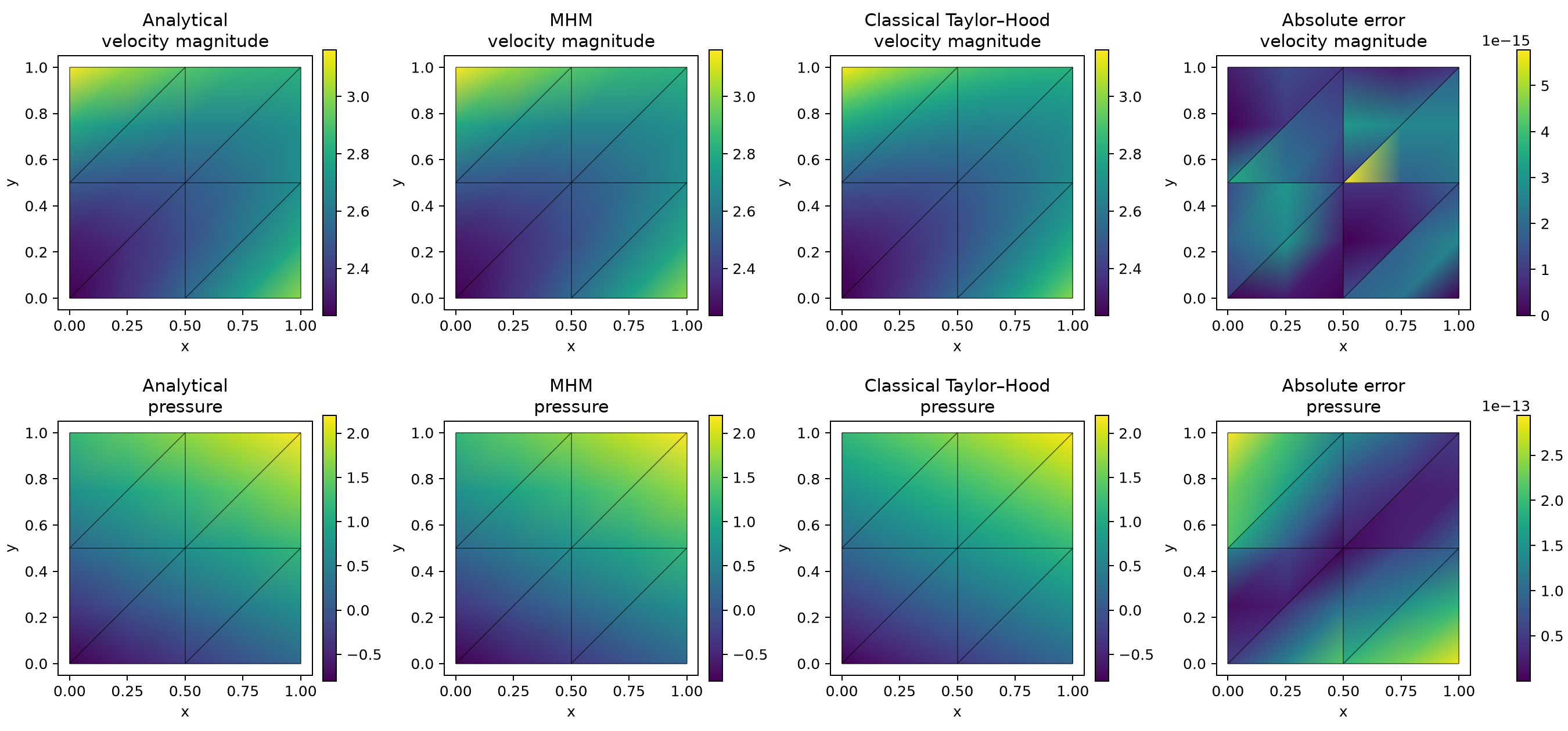
Every field panel includes the actual macro mesh. Incident reconstructions are evaluated independently.

7. Finish with a smooth asymptotic refinement family

The notebook next defines the smooth refinement problem explicitly, assembles its stabilized local and global equations, and plots the resulting fields. This second family keeps stabilized P3/P3 local fields, vector P1 traces and a crisscross macro mesh throughout refinement. Its local spaces and operator differ from the affine Taylor–Hood control above.

For that rate family the independently differentiated data are

\[ \begin{aligned} \psi&=-128x^2(1-x)^2y^2(1-y)^2, &u_*&=(\partial_y\psi,-\partial_x\psi),\\ p_*&=(x-y)^6-\tfrac1{28}, &\beta&=(1,1)/\sqrt2,\quad\nu=\gamma=1. \end{aligned} \]

The equal-order local form adds the Oseen residual and its adjoint convection sign, rather than using the Taylor–Hood form without stabilization:

\[ \begin{aligned} R(u,p)&=-\nu\Delta u+(\nabla u)\beta+\gamma u+\nabla p,\\ R^*(v,q)&=-\nu\Delta v-(\nabla v)\beta+\gamma v+\nabla q,\\ a_K^{\rm US}&=a_K+\sum_\tau\kappa_\tau(\nabla\cdot u,\nabla\cdot v)_\tau -\sum_\tau\delta_\tau(R(u,p),R^*(v,q))_\tau. \end{aligned} \]

Its load includes \(-\sum_\tau\delta_\tau(f,R^*(v,q))_\tau\). With the computed inverse constant \(m_\tau\), define \(d_\tau=4\nu/m_\tau\) and \(b_\tau=h_\tau\lVert\beta\rVert_\infty\):

\[ \delta_\tau=\frac{h_\tau^2} {\max(\gamma h_\tau^2,d_\tau)+\max(d_\tau,b_\tau)}, \qquad\kappa_\tau=b_\tau\min(1,b_\tau/d_\tau). \]

In the notebook, the source is differentiated symbolically from the physical solution, before compiling a form. The same function declares the stabilized local form and the unstabilized classical reference:

x = ufl.SpatialCoordinate(domain)
psi = -128*x[0]**2*(1-x[0])**2*x[1]**2*(1-x[1])**2
truth = ufl.as_vector((psi.dx(1), -psi.dx(0)))
truth_pressure = (x[0]-x[1])**6-1/28
beta = ufl.as_vector((1/np.sqrt(2), 1/np.sqrt(2)))
force = (-ufl.div(ufl.grad(truth))+ufl.grad(truth)*beta
         +truth+ufl.grad(truth_pressure))
residual = -ufl.div(ufl.grad(u))+ufl.grad(u)*beta+u+ufl.grad(p)
adjoint = -ufl.div(ufl.grad(v))-ufl.grad(v)*beta+v+ufl.grad(q)
a += (kappa*ufl.div(u)*ufl.div(v)-delta*ufl.inner(residual, adjoint))*dx
L = (ufl.inner(force, v)-delta*ufl.inner(force, adjoint))*dx

The tutorial computes the required local inverse constant using the shared finite-element tabulation and inverse-bound operations, then binds the displayed \(\delta_\tau\) and \(\kappa_\tau\) as native coefficient values. It declares the velocity and pressure fields, two retained velocity moments, negative velocity jump pairing and one global zero-mean pressure gauge explicitly. With eight macro grid subdivisions, its independently integrated velocity, pressure and product-norm errors are \(9.1431\times10^{-4}\), \(4.6453\times10^{-2}\) and \(7.9393\times10^{-2}\). The original uncondensed local and global equations have relative residual \(1.36\times10^{-14}\); the reconstructed pressure mean is within \(7.3\times10^{-16}\) of zero.

For the independent classical reference, the notebook sets \(\delta=\kappa=0\) and assembles the same physical UFL operator in globally conforming P2/P1 Taylor–Hood spaces, with strong zero exterior velocity and the same pressure gauge. Its own analytical errors decrease on three global meshes:

Global subdivisions	Velocity \(L^2\) error	Pressure \(L^2\) error	Product-norm error
16	\(6.7828\times10^{-4}\)	\(3.1377\times10^{-3}\)	\(8.3591\times10^{-2}\)
32	\(8.4786\times10^{-5}\)	\(3.0846\times10^{-4}\)	\(2.1030\times10^{-2}\)
64	\(1.0602\times10^{-5}\)	\(4.6421\times10^{-5}\)	\(5.2672\times10^{-3}\)

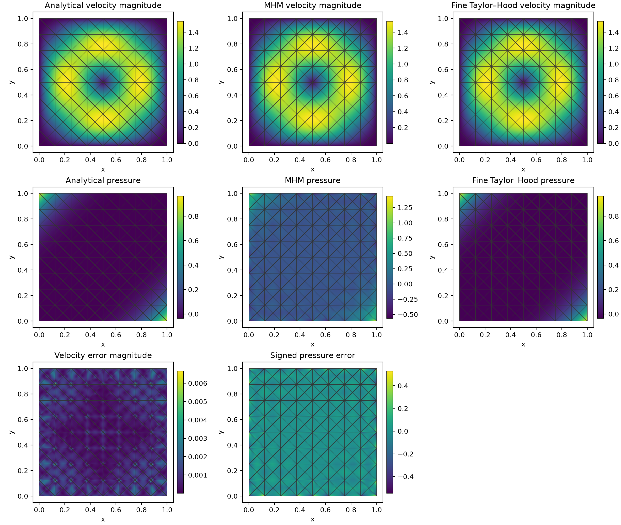
The reference is a numerical approximation. The MHM panels retain independent incident reconstructions and the actual crisscross macro mesh; the coarse pressure visualization exposes its larger interface errors rather than smoothing them away.

The direct literature comparison uses the product norm defined in Araya et al. (2021), Section 2.2:

\[ \begin{aligned} \lVert(e_u,e_p)\rVert_{V\times Q}^2 ={}&d_\Omega^{-2}\lVert e_u\rVert_{L^2(\Omega)}^2 +\sum_K\lVert\nabla e_u\rVert_{L^2(K)}^2 +\lVert e_p\rVert_{L^2(\Omega)}^2. \end{aligned} \]

For face degree one, Section 5.1 reports order two in this norm. The same observable is integrated here, with \(d_\Omega=\sqrt2\) on the unit square. The last three orders are \(2.0268\), \(2.0144\) and \(1.9991\). Pressure has orders \(2.0778\), \(2.0904\) and \(2.0549\), consistent with the published numerical product-norm orders. The separately plotted velocity \(L^2\) orders \(3.0692\), \(2.9885\) and \(2.9697\) are observed additional accuracy. Section 5.1 is a numerical study; the paper's Theorem 7 proves a posteriori reliability and efficiency under its hypotheses, rather than a third-order velocity \(L^2\) estimate.

The comparison assumes constant positive viscosity, full Dirichlet velocity, smooth data, a regular mesh family and positive effective reaction \(\gamma-\tfrac12\nabla\cdot\beta\). These conditions hold for this fixed coefficient example. Araya et al. (2021) state the coercivity and residual-test requirements; decreasing viscosity is a different parameter study.

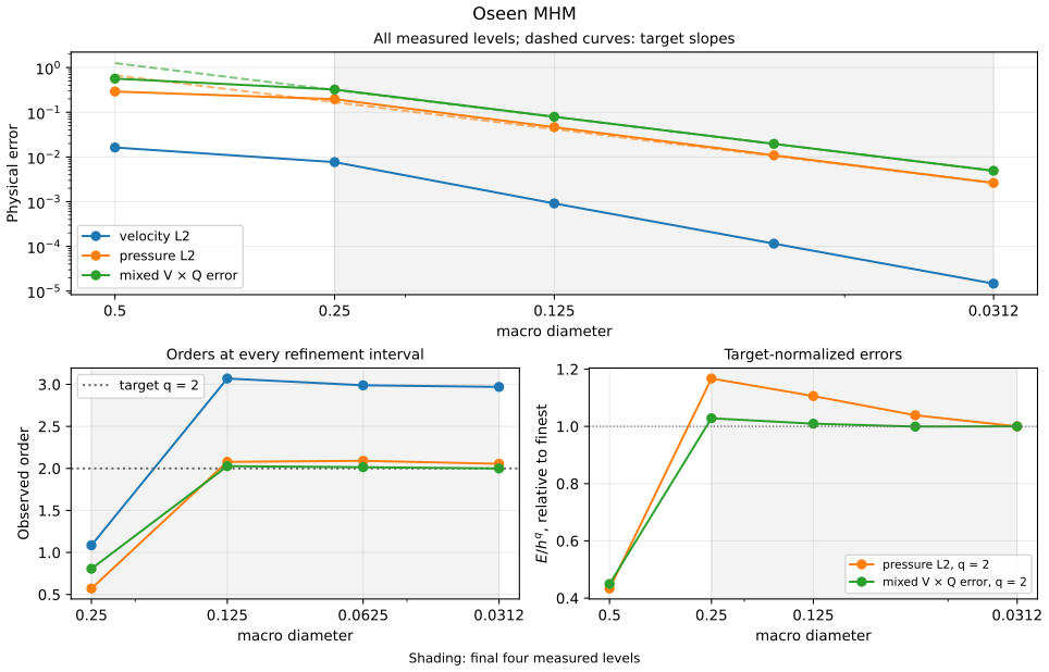
The notebook reads the attributed JSON acquisition, prints its SHA-256 source digest and computes consecutive rates. The flow gallery links the other current Oseen studies. This study qualifies the declared uniform mesh family; adaptive refinement is evaluated in the separate gallery studies.

References

• Rodolfo Araya, Cristian Cárcamo, Abner H. Poza and Frédéric Valentin (2021). An adaptive multiscale hybrid-mixed method for the Oseen equations. Advances in Computational Mathematics 47, article 15. DOI: 10.1007/s10444-020-09833-8.