MHM-USFEM: stabilized reaction–diffusion locals
Open the step-by-step notebook · Download notebook
Follow the numbered steps: state the variational problem, choose the local and trace spaces, declare the local and global equations, solve, and inspect the physical fields.
The main workflow is meshes → spaces → local equations → global balance → assemble → solve → fields and errors. MeshHierarchy associates macro and local meshes; bind_interface and LocalContext own supported numbering, geometric orientation and native coordinate conversions. The mathematical forms, physical trace meaning, local modes and gauge remain explicit in the cells below. Fully manual/custom spaces use the same numerical owners; see the custom-interface notebook.
We explicitly construct Equation, LocalEquations and MultiscaleProblem, then connect each code block to the physical formulation. MHM-USFEM is the name used here for scalar MHM-UNUSUAL of Martins, Pacazuca and Valentin (2025), Eqs. (14)–(15), §4.1. This is a scalar reaction–diffusion example; the separate Stokes–Brinkman tutorial treats velocity and pressure. Advection is zero here, and the negative residual stabilization is different from SUPG.
Open the downloaded notebook with jupyter lab after installing pymhm[notebooks,visualization] and the compatible native DOLFINx/UFL backend. Exact data, sources, local and global forms, boundary conditions, independent references, norms and plots are all defined below. PyMHM supplies generic UFL compilation, oriented trace integration, condensation and checked linear algebra.
We compare an intentionally underresolved P1/P0 control with a refined P1/P0 family that partitions each macroface and satisfies the paper's red-refinement condition. Both use the same physical equation and the published stabilization parameter. Reduced nodal oscillation can coexist with a larger integrated error; we report both. Our declared SW–NE connectivity, strong exterior Dirichlet enforcement and local meshes do not constitute a reproduction of the paper's historical figures.
The PyMHM distribution contains only the library. The first cell explicitly
downloads a checksum-verified companion archive and prepares the declared data
using its local Python helpers. You can inspect these support files in ROOT.
Complete studies and historical replay retain their existing opt-in flags.
from pathlib import Path
import os
import sys
from pymhm.io.workspace import workspace_from_archive

# Download verified support files; this operation does not execute them.
COMPANION_URL = "https://ipes-lncc.github.io/pymhm/downloads/e482bd3b768df30dca25cc72b5e147b051f60b59f6d8b7c0d87bc976b931b487/mhm_usfem_rad-companion.zip"
COMPANION_SHA256 = "e482bd3b768df30dca25cc72b5e147b051f60b59f6d8b7c0d87bc976b931b487"
WORKSPACE = Path(
    os.environ.get("PYMHM_WORKSPACE", Path.cwd() / ".pymhm-companions" / COMPANION_SHA256)
)
ROOT = workspace_from_archive(COMPANION_URL, sha256=COMPANION_SHA256, directory=WORKSPACE)
os.environ["PYMHM_WORKSPACE"] = str(ROOT)
if str(ROOT) not in sys.path:
    sys.path.insert(0, str(ROOT))

# Explicitly prepare declared data with the downloaded Python helpers.
from scripts.notebook_reproduction import notebook_workspace

ROOT = notebook_workspace("introduction/mhm_usfem_rad.ipynb", directory=ROOT)
root = ROOT
print("Workspace:", ROOT)


import json
import numpy as np
from pymhm import TriangleMesh, FaceSpace, SkeletonSpace
from pymhm.core.equations import Equation, LocalEquations
from pymhm.core.multiscale import assemble

REPORTS = ROOT / "build/introduction"
REPORTS.mkdir(parents=True, exist_ok=True)
np.set_printoptions(precision=5, suppress=True)
from pymhm.fem.scalar.triangle import nodal_space

from dataclasses import dataclass, replace
from typing import Any
from threadpoolctl import threadpool_limits

threadpool_limits(limits=1)
from pymhm import MeshHierarchy, LocalContext, bind_interface, bind_problem

from functools import partial
from examples.introduction.transport import (
    scalar_error_norms,
    scalar_reference,
    record_rad_case,
    plot_rad_primary,
    plot_rad_severe,
    plot_rad_refined,
    plot_rad_profiles,
)
from examples.introduction.vector import execution_provenance

measure_case = partial(record_rad_case, reports=REPORTS, root=ROOT)
Runtime resources (independent of the formulation)
The equations, approximation spaces, quadrature and error checks below do not depend on the worker count. We schedule independent local solves with ExecutionConfig; the coordinator adds their global contributions in a deterministic order, including contributions to shared faces. The conforming reference solves and postprocessing remain serial.
The default PYMHM_RAD_EXECUTION=auto runs small cases serially. It selects processes for the resolved family when there are at least 512 macroelements, eight local subdivisions and four face segments. This choice follows a representative timing control for this tutorial, rather than a general performance claim. The default upper bound is 32 workers, limited by this process's CPU affinity. Set PYMHM_RAD_WORKERS to override that upper bound, or PYMHM_RAD_EXECUTION=serial, thread or process to explicitly select a backend. Passing an ExecutionConfig directly to solve_rad_case bypasses the automatic choice.
Each worker uses one native BLAS/OpenMP thread. A bounded pipeline holds at most twice the active worker count in flight, and each solve caps the active worker count at its number of macroelements. These options change execution resources only.
A notebook-owned temporary directory holds the local UFL compiler cache. For every solve configuration, we assemble the first two macrotriangles serially before starting workers: these triangles cover the two orientations in this mesh. This warms the volume and face kernels for the chosen diffusion, stabilization and face partition. The optional process worker module below is generated in this same owned directory from the notebook's functions. The cache remains alive throughout the study and is removed after the final result is saved. The 7200-second compiler timeout is not a solver tolerance.
After the final cleanup, rerun both the runtime-resource and worker-export cells before solving again. If the study is interrupted, let PyMHM finish releasing its workers, then call RAD_JIT_CACHE.cleanup() or restart the kernel before restarting the setup.
from tempfile import TemporaryDirectory
from pymhm.execution.cpu import ExecutionConfig

try:
    RAD_AVAILABLE_CPUS = len(os.sched_getaffinity(0))
except (AttributeError, OSError):
    RAD_AVAILABLE_CPUS = os.cpu_count() or 1

RAD_POLICY = os.environ.get("PYMHM_RAD_EXECUTION", "auto")
if RAD_POLICY not in {"auto", "serial", "thread", "process"}:
    raise ValueError("PYMHM_RAD_EXECUTION must be 'auto', 'serial', 'thread', or 'process'")
RAD_WORKERS = int(os.environ.get("PYMHM_RAD_WORKERS", str(min(32, RAD_AVAILABLE_CPUS))))
RAD_EXECUTION = ExecutionConfig(
    backend="process" if RAD_POLICY == "auto" else RAD_POLICY,
    workers=RAD_WORKERS,
    native_threads=1,
    batch_size=2 * RAD_WORKERS,
    pipeline=True,
)
RAD_JIT_CACHE = TemporaryDirectory(prefix="pymhm-rad-jit-")
RAD_JIT_OPTIONS = {"cache_dir": Path(RAD_JIT_CACHE.name), "timeout": 7200}
print(
    "Local execution policy:", RAD_POLICY,
    "workers:", RAD_EXECUTION.effective_workers,
    "native threads per worker:", RAD_EXECUTION.native_threads,
    "pending bound:", RAD_EXECUTION.effective_batch_size,
)
1. Identify the equation, boundary data and difficult length scale
On the unit square, reaction and source are one and diffusion is a positive constant:
The exact solution has two layers with width of order \(\sqrt\epsilon\):
Differentiating gives \(-\epsilon u''+u=1\), independently of the discrete operator. At \(\epsilon=10^{-5}\), a coarse uniform local mesh cannot resolve the layer. We measure nodal overshoot above the physical upper bound one, nodal error and integrated errors. The coarse control keeps the same spaces as diffusion decreases; a separate resolution family tests whether the physical fields improve when both the local and trace approximation spaces are refined.
@dataclass(frozen=True)
class ReactionLayer:
    """Equation (22): ``-epsilon*Delta u+u=1`` with vertical zero Dirichlet data.

    Horizontal boundaries carry zero outward physical flux ``-epsilon*grad(u).n``.
    ``epsilon`` is positive and the layer width is its square root. Evaluation
    avoids positive exponential arguments, including in very thin layers.
    """

    epsilon: float

    def __post_init__(self) -> None:
        """Require a finite positive physical diffusion coefficient."""
        if not np.isfinite(self.epsilon) or self.epsilon <= 0:
            raise ValueError("epsilon must be finite and positive")

    def value(self, points: np.ndarray) -> np.ndarray:
        """Evaluate the exact scalar on physical unit-square coordinates."""
        scale = 1 / np.sqrt(self.epsilon)
        x = points[:, 0]
        return 1 - (np.exp(-scale * x) + np.exp(-scale * (1 - x))) / (1 + np.exp(-scale))

    def gradient(self, points: np.ndarray) -> np.ndarray:
        """Evaluate the independently differentiated physical gradient."""
        scale = 1 / np.sqrt(self.epsilon)
        x = points[:, 0]
        derivative = scale * (np.exp(-scale * x) - np.exp(-scale * (1 - x))) / (1 + np.exp(-scale))
        return np.column_stack((derivative, np.zeros(len(points))))
EPSILON = 1e-3
# This scientific family fixes scalar P1 and multiplier P0.
LOCAL_SUBDIVISIONS = 2
LOCAL_QUADRATURE_DEGREE, OPERATOR_CHECK_ORDER, ERROR_ORDER = 8, 12, 24
truth = ReactionLayer(EPSILON)

# The independently differentiated equation is -epsilon*u'' + u = 1.
x = np.linspace(0, 1, 101)
points = np.column_stack((x, np.full_like(x, 0.37)))
scale = 1 / np.sqrt(EPSILON)
second = -(scale**2) * (np.exp(-scale * x) + np.exp(-scale * (1 - x))) / (1 + np.exp(-scale))
np.testing.assert_allclose(-EPSILON * second + truth.value(points), 1, atol=2e-15)
np.testing.assert_allclose(truth.gradient(points)[:, 1], 0)
2. Write the local equations and skeletal balance
Let \(B_K\) integrate the globally oriented flux basis against the trace of a local test function. In the matrix equations below, \(u_K\) is the local scalar coefficient vector and \(\lambda\) is the global trace coefficient vector; their basis evaluations give the physical scalar and flux multiplier. The API expresses
Summing the \(C_Ku_K\) equations imposes continuity of scalar trace moments on internal faces. The normal interface binding supplies the two opposite incident orientations; b and c are declared independently with UFL boundary forms. On active flux faces, \(\lambda=q\cdot n_F\) uses a single global face normal; with zero advection there is no Robin correction to the physical diffusive flux.
The complete strong reaction–diffusion operator is \(Lw=w-\epsilon\Delta w\). USFEM changes the local bilinear and linear forms:
Locals are P1, hence \(\Delta v_h=0\) inside each fine triangle and \(Lv_h=v_h\). This justifies the published \(m=1/3\) for this space. Below we declare the Galerkin form directly in UFL, then add the negative residual form and its matching source. assemble_form executes native assembly; the native space binding owns the coefficient convention, while context trace pairings supply the declared UFL interface integrals.
Reaction makes the local operator invertible: constants are not a kernel, and no retained coarse amplitudes are required. On vertical exterior faces, zero scalar data are imposed strongly by removing their nodal coordinates and exterior flux columns. Horizontal exterior faces prescribe zero normal flux. Vertical Dirichlet faces are absent from flux coupling: their zero dummy trace coordinates do not prescribe the physical flux. The global balance is tested on the free internal trace coordinates.
For P1/P0 in two dimensions, Theorem 1 requires one red refinement of a simplicial local mesh that matches the macroface partition. With one P0 segment per macroface, two local subdivisions meet this condition. With four P0 segments per face, we declare a matching uniform four-subdivision mesh and take its red refinement: eight local subdivisions. This condition concerns compatibility of the trace and local spaces; a positive local matrix alone does not establish global stability.
import basix.ufl
import dolfinx
import ufl


def rad_forms(domain: Any, *, epsilon: float, stabilized: bool) -> tuple[Any, Any, Any]:
    """Translate the local reaction–diffusion bilinear form and load into UFL."""
    V = dolfinx.fem.functionspace(domain, basix.ufl.element("Lagrange", "triangle", 1))
    u, v = ufl.TrialFunction(V), ufl.TestFunction(V)
    dx = ufl.Measure("dx", domain=domain, metadata={"quadrature_degree": LOCAL_QUADRATURE_DEGREE})
    a = (epsilon * ufl.inner(ufl.grad(u), ufl.grad(v)) + u * v) * dx
    L = v * dx
    if stabilized:
        Lu, Lv = u - epsilon * ufl.div(ufl.grad(u)), v - epsilon * ufl.div(ufl.grad(v))
        h = ufl.CellDiameter(domain)
        tau = (h**2 / 3) / (ufl.max_value(h**2 / 3, 2 * epsilon) + 2 * epsilon)
        a -= tau * Lu * Lv * dx
        L -= tau * Lv * dx
    return V, a, L
The native mesh and coefficient conversions come from the shared backend binding. The provider below writes the volume and boundary forms, chooses its physical boundary conditions and registers the scalar field. The explicit restriction to free scalar coordinates imposes the declared vertical Dirichlet data; it is part of the formulation.
import basix


from pymhm.backends.spaces import create_native_mesh
from pymhm.backends.forms import assemble_form, assemble_pairing
LocalEquations now receives the executed forms through the shared native-space binding. LocalContext owns the mesh and interface maps. The following provider applies the vertical Dirichlet nodes, keeps the horizontal physical-flux convention, and exposes the two oriented trace blocks directly.
def local_rad(
    local: LocalContext,
    *,
    macro: TriangleMesh,
    skeleton: SkeletonSpace,
    epsilon: float,
    stabilized: bool,
    local_subdivisions: int = LOCAL_SUBDIVISIONS,
) -> LocalEquations:
    """Declare and execute the local scalar UFL form, then apply explicit mixed data."""
    fine = local.mesh
    domain = create_native_mesh(fine)
    V, a, L = rad_forms(domain, epsilon=epsilon, stabilized=stabilized)
    # Generic native assembly and coordinate permutation, independent of the PDE.
    binding = local.native_space(V)
    order = binding.mapping
    native_A = assemble_form(a, jit_options=RAD_JIT_OPTIONS)
    native_F = assemble_form(L, jit_options=RAD_JIT_OPTIONS)
    A, F = native_A[order][:, order], native_F[order]
    _, nodes = nodal_space(fine, 1)
    u, v = ufl.TrialFunction(V), ufl.TestFunction(V)
    pair_b = local.trace_pairings(lambda phi, ds: phi * v * ds)
    pair_c = local.trace_pairings(lambda phi, ds: -phi * u * ds, axis="rows")
    B = assemble_pairing(
        pair_b.forms, axis="columns", jit_options=RAD_JIT_OPTIONS
    )[order]
    C = assemble_pairing(
        pair_c.forms, axis="rows", jit_options=RAD_JIT_OPTIONS
    )[:, order]
    fixed_nodes = np.flatnonzero(
        np.isclose(nodes[:, 0], 0, atol=1e-12) | np.isclose(nodes[:, 0], 1, atol=1e-12)
    )
    free = np.setdiff1d(np.arange(len(nodes)), fixed_nodes)
    local.field("scalar", binding, reconstruction=binding.to_native(np.eye(len(nodes))[:, free]))
    B, C = B[free], C[:, free]
    return local.equations(
        a=A[free][:, free],
        L=F[free],
        b=B,
        c=C,
        metadata={
            "mesh": fine,
            "free": free,
            "nodes": len(nodes),
            "local_subdivisions": local_subdivisions,
        },
    )
Optional runtime setup: importable functions for spawned workers
The mathematical definitions above are the complete local formulation. The next cell concerns Python process execution only: a spawned worker must import its callable from a module, whereas a notebook function lives in an interactive session.
We use inspect.getsource to export the exact functions just defined above, their imports and the declared constants to a temporary module. There is no second maintained copy of the operator or stabilization. PyMHM still owns process scheduling, local elimination, ordered assembly and native resource cleanup. You can select serial or thread execution with the same mathematical functions; those modes use the original notebook functions directly.
The module name identifies the complete generated source payload. If you edit a function or constant and rerun this cell, workers import the new implementation rather than a previously imported notebook callback.
import hashlib
import importlib
import inspect

RAD_PROVIDER_SOURCE = "\n\n".join(
    inspect.getsource(function).rstrip() for function in (rad_forms, local_rad)
)
RAD_WORKER_IMPORTS = """from pathlib import Path
from typing import Any
import numpy as np
import basix.ufl
import dolfinx
import ufl
from pymhm import TriangleMesh, SkeletonSpace, LocalContext
from pymhm.core.equations import LocalEquations
from pymhm.fem.scalar.triangle import nodal_space
from pymhm.backends.spaces import create_native_mesh
from pymhm.backends.forms import assemble_form, assemble_pairing
"""
RAD_WORKER_CONSTANTS = (
    f"LOCAL_SUBDIVISIONS = {LOCAL_SUBDIVISIONS!r}\n"
    f"LOCAL_QUADRATURE_DEGREE = {LOCAL_QUADRATURE_DEGREE!r}\n"
    f"RAD_JIT_OPTIONS = {{'cache_dir': Path({RAD_JIT_CACHE.name!r}), 'timeout': 7200}}\n"
)
RAD_WORKER_PAYLOAD = (
    RAD_WORKER_IMPORTS + "\n" + RAD_WORKER_CONSTANTS + "\n" + RAD_PROVIDER_SOURCE + "\n"
)
RAD_WORKER_MODULE_NAME = (
    "_pymhm_rad_workers_" + hashlib.sha256(RAD_WORKER_PAYLOAD.encode()).hexdigest()
)
RAD_WORKER_FILE = Path(RAD_JIT_CACHE.name) / (RAD_WORKER_MODULE_NAME + ".py")
RAD_WORKER_FILE.write_text(RAD_WORKER_PAYLOAD, encoding="utf-8")
sys.path.insert(0, RAD_JIT_CACHE.name)
importlib.invalidate_caches()
RAD_WORKER_MODULE = importlib.import_module(RAD_WORKER_MODULE_NAME)
RAD_PROVIDER_SOURCE_SHA256 = hashlib.sha256(RAD_PROVIDER_SOURCE.encode()).hexdigest()
print("Spawned workers import the notebook's exact provider source:", RAD_PROVIDER_SOURCE_SHA256)
Spawned workers import the notebook's exact provider source: b0215d50091b1728a47c15d81a7439bd30101d9771889e373d002dc90c086766
The primary operator above is the executed UFL form. As a secondary convenience check, scalar_operators can assemble its unstabilized part. We compare its restricted matrix and load against our declared Galerkin equation on one representative macrocell; it is not used to define the tutorial's MHM operators.
from pymhm.fem.scalar.triangle import scalar_operators

probe_macro = TriangleMesh.unit_square(2)
probe_skeleton = SkeletonSpace(probe_macro, tuple(FaceSpace.uniform(0) for _ in probe_macro.faces))
probe_problem = bind_problem(
    MeshHierarchy(
        probe_macro,
        tuple(
            probe_macro.submesh(cell, LOCAL_SUBDIVISIONS) for cell in range(len(probe_macro.cells))
        ),
    ),
    bind_interface(probe_skeleton, convention="normal"),
    lambda local: local_rad(
        local, macro=probe_macro, skeleton=probe_skeleton, epsilon=EPSILON, stabilized=False
    ),
)
probe_equation = probe_problem.local_provider(0)
ready_A, _, ready_F = scalar_operators(
    probe_equation.metadata["mesh"],
    1,
    diffusion=EPSILON,
    reaction=1.0,
    source=1.0,
    order=OPERATOR_CHECK_ORDER,
)
free = probe_equation.metadata["free"]
np.testing.assert_allclose(probe_equation.a.toarray(), ready_A[free][:, free].toarray(), atol=1e-14)
np.testing.assert_allclose(probe_equation.L, ready_F[free], atol=1e-14)
3. Declare and solve the global problem
Equation(0,0) adds zero to the sum of the local balances. Homogeneous boundary data already enter the local restrictions and fixed exterior trace coefficients. assemble eliminates each independent local operator; the global solve then reconstructs the local coefficients. No call selects a PDE from a model name.
We measure the broken scalar error and physical flux \(-\epsilon\nabla u_h\) against the analytical fields. The following quadrature utility also records nodal extrema, since a small integral error alone can miss oscillations in a thin layer.
Norm integration, archive replay and field/profile displays are importable from examples/introduction/transport.py and examples/introduction/vector.py. The local forms and the complete global solve remain above; the conforming P2 forms below are separately declared.
Record the numerical coordinates for reproducibility
The next utility saves the actual local coordinate basis, coefficients, orientation maps and reconstructed fields as each solve finishes. It contains no physical operator. Replaying the saved basis is checked with one and two BLAS threads; this positive-reaction example has no local nullspace modes. You can read the global construction immediately below without studying the archive format first.
def solve_rad_case(
    n,
    epsilon,
    stabilized,
    *,
    face_subdivisions=1,
    local_subdivisions=LOCAL_SUBDIVISIONS,
    execution: ExecutionConfig | None = None,
):
    """Declare the mesh, multiplier space and scalar global equation for one configuration."""
    macro = TriangleMesh.unit_square(n)
    skeleton = SkeletonSpace(
        macro, tuple(FaceSpace.uniform(0, face_subdivisions) for _ in macro.faces)
    )
    if execution is None:
        execution = RAD_EXECUTION
        resolved_parallel_case = (
            len(macro.cells) >= 512 and local_subdivisions >= 8 and face_subdivisions >= 4
        )
        if RAD_POLICY == "auto" and not resolved_parallel_case:
            execution = replace(execution, backend="serial")
    local_workers = min(execution.effective_workers, len(macro.cells))
    case_execution = replace(
        execution,
        workers=local_workers,
        batch_size=min(execution.effective_batch_size, 2 * local_workers),
    )
    local_function = (
        RAD_WORKER_MODULE.local_rad if execution.backend == "process" else local_rad
    )
    provider = partial(
        local_function,
        macro=macro,
        skeleton=skeleton,
        epsilon=epsilon,
        stabilized=stabilized,
        local_subdivisions=local_subdivisions,
    )
    hierarchy = MeshHierarchy(
        macro, tuple(macro.submesh(c, local_subdivisions) for c in range(len(macro.cells)))
    )
    # Vertical scalar data are strong in local_rad; horizontal physical flux is zero.
    fixed = {int(d): 0.0 for f in macro.boundary_faces for d in skeleton.dofs(int(f))}
    problem = bind_problem(
        hierarchy,
        bind_interface(skeleton, convention="normal"),
        provider,
        global_equation=Equation(0, 0),
        retained=0,
        fixed=fixed,
    )
    # Compile both triangle orientations on the coordinator before starting workers.
    # This covers this coefficient/stabilization/face-partition configuration.
    for cell in range(min(2, len(macro.cells))):
        problem.local_provider(cell)
    system = assemble(problem, execution=case_execution)
    return macro, skeleton, system, system.solve()


METHODS = (("MHM-Galerkin", False), ("MHM-USFEM", True))
cases, rows, state_archives = {}, [], []
for n in (2, 4, 8, 16):
    for method, stabilized in METHODS:
        case, row, archive = measure_case(
            *solve_rad_case(n, EPSILON, stabilized),
            truth,
            order=ERROR_ORDER,
            name=f"rad-n{n}-{method.lower().replace(' ', '-')}",
            named=True,
            method=method,
            n=n,
            H=1 / n,
        )
        cases[n, method] = case
        rows.append(row)
        state_archives.append(archive)
rows
Numerical output and provenance
[{'macro_cells': 8,
  'fine_cells': 32,
  'trace_dofs': 16,
  'residual': 2.043158148055947e-18,
  'scalar_l2': 0.25331511823245645,
  'flux_l2': 0.0049922958737293735,
  'gradient_l2': 4.992295873729374,
  'scalar_relative_l2': 0.26625957192826877,
  'nodal_error': 0.37771283714762327,
  'nodal_minimum': 0.0,
  'nodal_maximum': 1.3773441986275734,
  'method': 'MHM-Galerkin',
  'n': 2,
  'H': 0.5},
 {'macro_cells': 8,
  'fine_cells': 32,
  'trace_dofs': 16,
  'residual': 1.0314124678157315e-17,
  'scalar_l2': 0.34175259280093,
  'flux_l2': 0.004894176612566581,
  'gradient_l2': 4.89417661256658,
  'scalar_relative_l2': 0.35921621930614284,
  'nodal_error': 0.19714623568561518,
  'nodal_minimum': 0.0,
  'nodal_maximum': 1.1126151697555124,
  'method': 'MHM-USFEM',
  'n': 2,
  'H': 0.5},
 {'macro_cells': 32,
  'fine_cells': 128,
  'trace_dofs': 56,
  'residual': 2.3581389225557654e-18,
  'scalar_l2': 0.12112741146990827,
  'flux_l2': 0.004115878117983086,
  'gradient_l2': 4.115878117983086,
  'scalar_relative_l2': 0.12731704665633647,
  'nodal_error': 0.25980313859039594,
  'nodal_minimum': 0.0,
  'nodal_maximum': 1.240603178434425,
  'method': 'MHM-Galerkin',
  'n': 4,
  'H': 0.25},
 {'macro_cells': 32,
  'fine_cells': 128,
  'trace_dofs': 56,
  'residual': 7.655488364338492e-18,
  'scalar_l2': 0.18208673599128516,
  'flux_l2': 0.004130825618653842,
  'gradient_l2': 4.130825618653842,
  'scalar_relative_l2': 0.19139140497080442,
  'nodal_error': 0.19374192827725978,
  'nodal_minimum': 0.0,
  'nodal_maximum': 1.1294675135664094,
  'method': 'MHM-USFEM',
  'n': 4,
  'H': 0.25},
 {'macro_cells': 128,
  'fine_cells': 512,
  'trace_dofs': 208,
  'residual': 4.5916800562639076e-18,
  'scalar_l2': 0.04656879012655305,
  'flux_l2': 0.002786462852626926,
  'gradient_l2': 2.786462852626926,
  'scalar_relative_l2': 0.048948464706062345,
  'nodal_error': 0.14438737561256298,
  'nodal_minimum': 0.0,
  'nodal_maximum': 1.125187415456592,
  'method': 'MHM-Galerkin',
  'n': 8,
  'H': 0.125},
 {'macro_cells': 128,
  'fine_cells': 512,
  'trace_dofs': 208,
  'residual': 1.1365012103379582e-17,
  'scalar_l2': 0.07656209768491802,
  'flux_l2': 0.002909494311749462,
  'gradient_l2': 2.909494311749462,
  'scalar_relative_l2': 0.08047443633747027,
  'nodal_error': 0.15551401548096855,
  'nodal_minimum': 0.0,
  'nodal_maximum': 1.1010938058504158,
  'method': 'MHM-USFEM',
  'n': 8,
  'H': 0.125},
 {'macro_cells': 512,
  'fine_cells': 2048,
  'trace_dofs': 800,
  'residual': 1.1955824945521019e-17,
  'scalar_l2': 0.016280778118692305,
  'flux_l2': 0.0017204001144176615,
  'gradient_l2': 1.7204001144176615,
  'scalar_relative_l2': 0.01711272916827719,
  'nodal_error': 0.15620122915430557,
  'nodal_minimum': 0.0,
  'nodal_maximum': 1.0320779526335582,
  'method': 'MHM-Galerkin',
  'n': 16,
  'H': 0.0625},
 {'macro_cells': 512,
  'fine_cells': 2048,
  'trace_dofs': 800,
  'residual': 1.4707313764539898e-17,
  'scalar_l2': 0.020197431303050736,
  'flux_l2': 0.0017279805508186468,
  'gradient_l2': 1.7279805508186468,
  'scalar_relative_l2': 0.02122952412128032,
  'nodal_error': 0.1212762367189939,
  'nodal_minimum': 0.0,
  'nodal_maximum': 1.0296587301268465,
  'method': 'MHM-USFEM',
  'n': 16,
  'H': 0.0625}]
4. Independently assemble and refine a classical conforming reference
The CG2 reference uses the same diffusion, unit reaction/source and mixed boundary data, with a globally conforming field and no skeleton or stabilization. Its real UFL form is independently assembled by DOLFINx below. We impose zero scalar values strongly on the vertical boundary and leave the horizontal zero-flux condition natural.
The exact solution lets us verify true reference errors on several fine meshes. For the severe \(\epsilon=10^{-5}\) challenge, additional meshes have 256, 512 and 1024 divisions in the layer-normal direction and 16 in the invariant direction. This declared anisotropy resolves the physical scale without changing the operator or boundary data. A numerical reference remains a numerical field, even when an exact field is also available.
def classical_rad_forms(space, epsilon):
    """Declare the separate conforming P2 operator, source and exact field."""
    u, v = ufl.TrialFunction(space), ufl.TestFunction(space)
    domain = space.ufl_domain()
    dx = ufl.Measure("dx", domain=domain, metadata={"quadrature_degree": 20})
    a = (epsilon * ufl.inner(ufl.grad(u), ufl.grad(v)) + u * v) * dx
    x = ufl.SpatialCoordinate(domain)
    exact = 1 - (ufl.exp(-x[0] / np.sqrt(epsilon)) + ufl.exp(-(1 - x[0]) / np.sqrt(epsilon))) / (
        1 + np.exp(-1 / np.sqrt(epsilon))
    )
    return a, v * dx, exact, dx


reference_rows, references = [], {}
REFERENCE_GRIDS = [(EPSILON, n, n) for n in (32, 64, 128)] + [
    (1e-5, n, 16) for n in (256, 512, 1024)
]
for epsilon, nx, ny in REFERENCE_GRIDS:
    case, row, archive = scalar_reference(
        epsilon, nx, ny, classical_rad_forms, ReactionLayer(epsilon), reports=REPORTS, root=ROOT
    )
    references[epsilon, nx] = case
    reference_rows.append(row)
    state_archives.append(archive)
5. Inspect fields and observed convergence rates
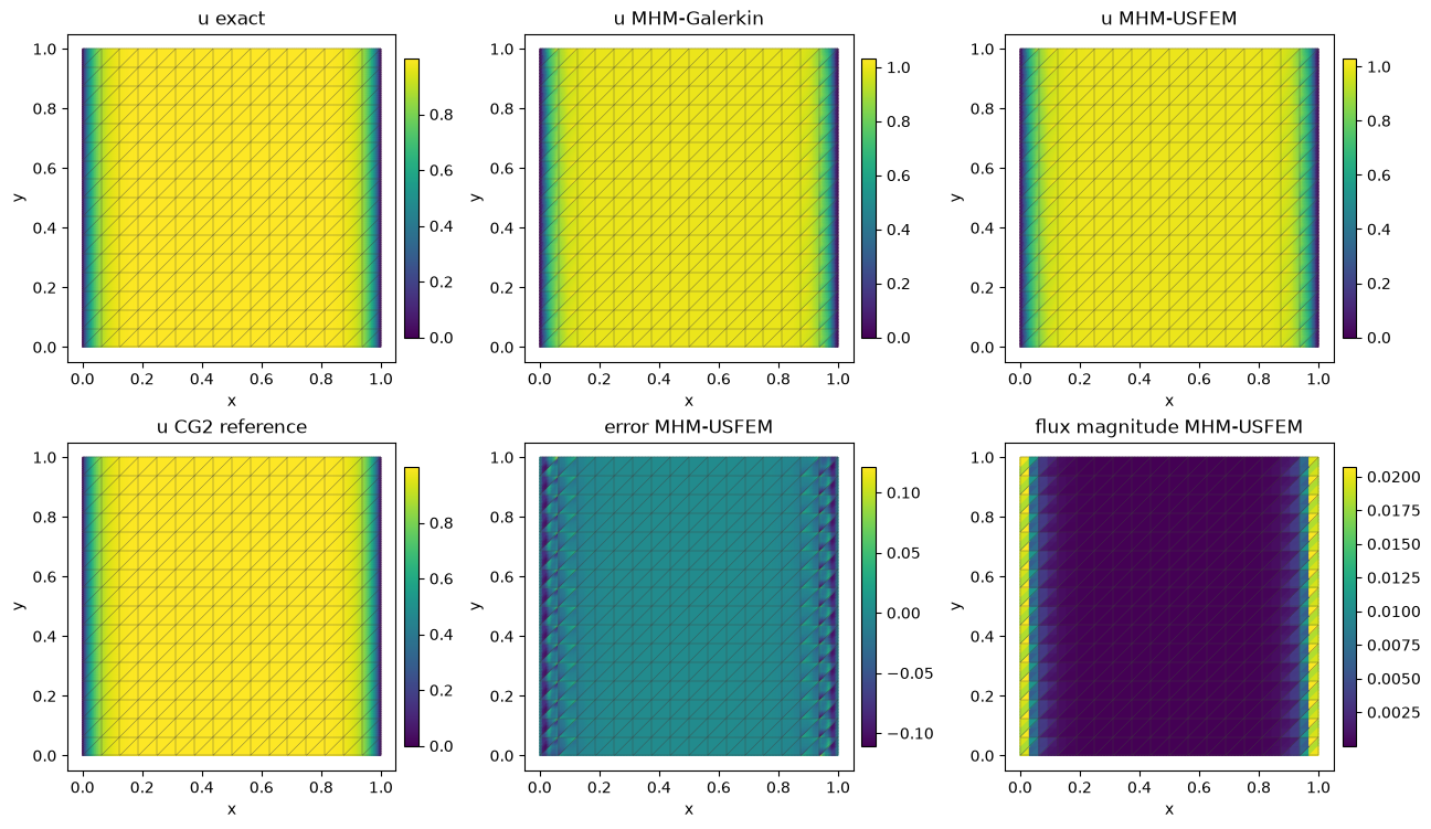
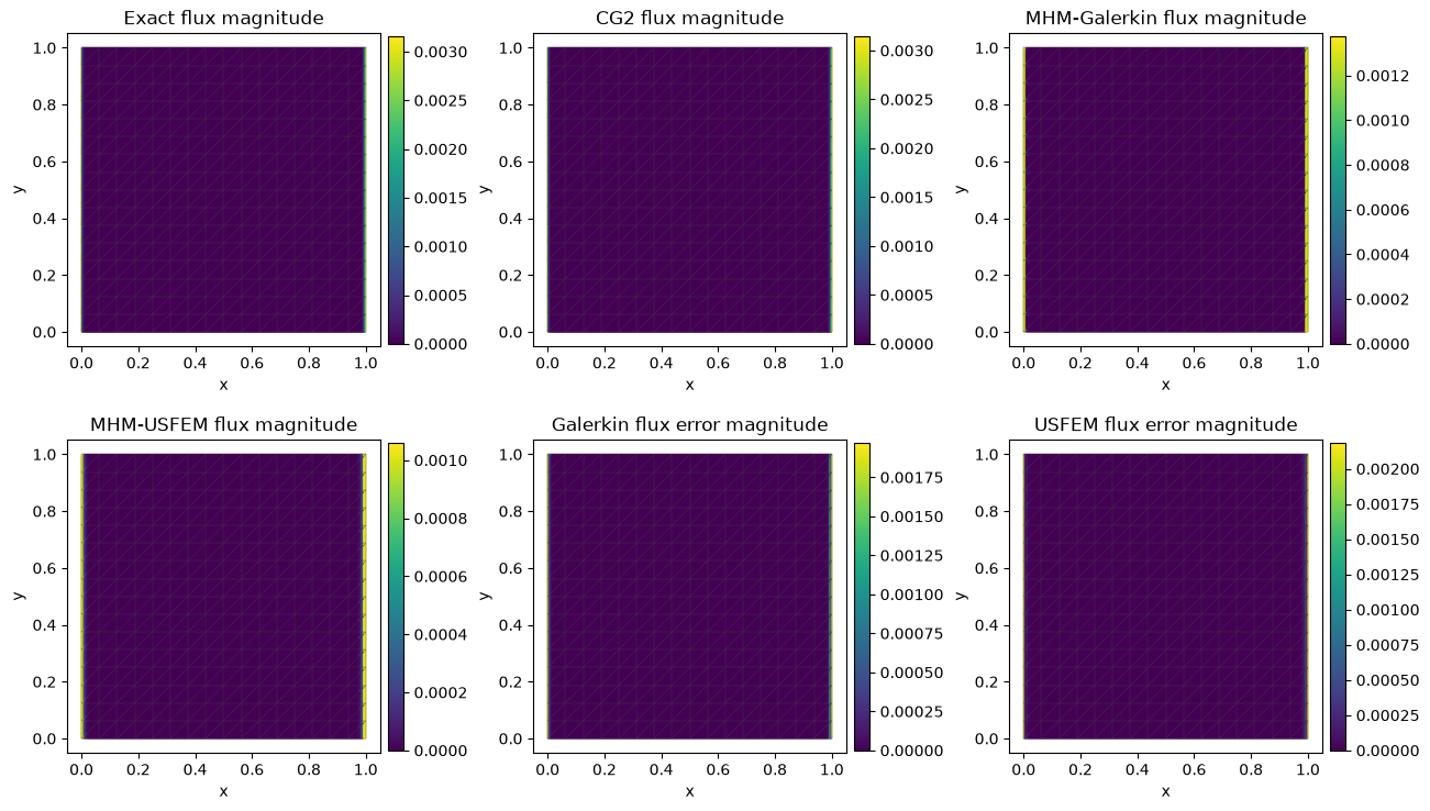
Every spatial panel highlights the actual MHM macro mesh, including analytical and reference panels. Flux means the raw physical field \(-\epsilon\nabla u_h\); the skeletal solve does not make it an H(div) reconstruction.
The sequence keeps P1 locals, P0 faces and two local subdivisions per macro edge, varying only the macro mesh. Reported rates are measured from this layer problem; smooth-problem orders are not assumed. Reference errors are measured separately against the exact solution.
For two successive resolutions, the measured slope is \(r=\log(e_1/e_2)/\log(H_1/H_2)\). These small plotting utilities compute that quantity directly and keep error and rate axes separate.
The display utility evaluates each local polynomial independently, including its one-sided boundary values. Every panel overlays the actual macro mesh and has its own color scale. It changes only the display sampling.
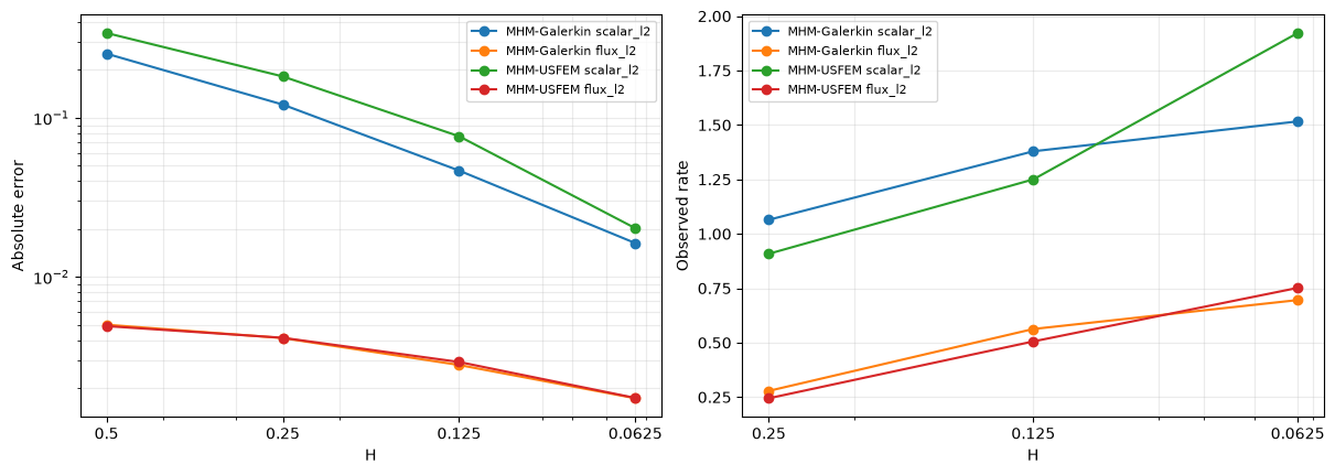
MHM-Galerkin scalar_l2 rates: [1.06441 1.37909 1.51619]
MHM-Galerkin flux_l2 rates: [0.2785  0.56277 0.69569]
MHM-USFEM scalar_l2 rates: [0.90833 1.24992 1.92246]
MHM-USFEM flux_l2 rates: [0.24464 0.50566 0.75168]
6. Preserve a deliberately underresolved control
Fix the macro mesh at \(n=8\), with one P0 segment per macroface and two local subdivisions. Both methods use the same scalar PDE and approximation spaces. Decreasing \(\epsilon\) makes the physical layer thinner without increasing resolution. This control demonstrates the approximation limits of these spaces.
For constant diffusion and P1 locals, the elementwise Laplacian vanishes. On the uniform fine mesh, write \(\eta=1-\tau\). The stabilized matrix and source reduce exactly to
Here \(K\) and \(M\) are the ordinary P1 stiffness and mass matrices. In the reaction-dominated branch, dividing by \(\eta\) exposes the discrete diffusion scale
This identity explains why the underresolved stabilized profile can have a broader transition. It does not change the physical diffusion or justify changing the method parameter. For this control, \(h_T=\sqrt{2}/16\approx0.0884\), whereas the physical layer width at \(\epsilon=10^{-5}\) is \(\sqrt{\epsilon}\approx0.00316\).
The tables keep overshoot, nodal error, scalar L2 and physical-flux L2 visible. USFEM need not improve every measure or preserve nodal bounds. The profiles retain independent one-sided values at every macroface intersection.
sweep, challenging = [], {}
macro = TriangleMesh.unit_square(8)
for epsilon in dict.fromkeys((1e-2, EPSILON, 1e-5)):
    for method, stabilized in METHODS:
        case, row, archive = measure_case(
            *solve_rad_case(8, epsilon, stabilized),
            ReactionLayer(epsilon),
            order=40,
            name=f"rad-eps{epsilon:g}-{method.lower()}",
            epsilon=epsilon,
            method=method,
        )
        row["overshoot"] = max(0.0, row["nodal_maximum"] - 1)
        challenging[epsilon, method] = case[2:]
        sweep.append(row)
        state_archives.append(archive)
sweep
Numerical output and provenance
[{'macro_cells': 128,
  'fine_cells': 512,
  'trace_dofs': 208,
  'residual': 2.821967046147381e-17,
  'scalar_l2': 0.015727506798012398,
  'flux_l2': 0.006979403304451645,
  'gradient_l2': 0.6979403304451645,
  'scalar_relative_l2': 0.018796381471541435,
  'nodal_error': 0.10172873787639769,
  'nodal_minimum': 0.0,
  'nodal_maximum': 0.9937189825987042,
  'epsilon': 0.01,
  'method': 'MHM-Galerkin',
  'overshoot': 0.0},
 {'macro_cells': 128,
  'fine_cells': 512,
  'trace_dofs': 208,
  'residual': 3.779329480464003e-17,
  'scalar_l2': 0.01684209049020335,
  'flux_l2': 0.006964009814822497,
  'gradient_l2': 0.6964009814822497,
  'scalar_relative_l2': 0.02012845148934158,
  'nodal_error': 0.08559220444620463,
  'nodal_minimum': 0.0,
  'nodal_maximum': 0.9909556114252319,
  'epsilon': 0.01,
  'method': 'MHM-USFEM',
  'overshoot': 0.0},
 {'macro_cells': 128,
  'fine_cells': 512,
  'trace_dofs': 208,
  'residual': 4.5916800562639076e-18,
  'scalar_l2': 0.046568790126552975,
  'flux_l2': 0.0027864628526269347,
  'gradient_l2': 2.7864628526269346,
  'scalar_relative_l2': 0.04894846470606227,
  'nodal_error': 0.14438737561256298,
  'nodal_minimum': 0.0,
  'nodal_maximum': 1.125187415456592,
  'epsilon': 0.001,
  'method': 'MHM-Galerkin',
  'overshoot': 0.12518741545659196},
 {'macro_cells': 128,
  'fine_cells': 512,
  'trace_dofs': 208,
  'residual': 1.1365012103379582e-17,
  'scalar_l2': 0.07656209768491792,
  'flux_l2': 0.0029094943117494707,
  'gradient_l2': 2.9094943117494707,
  'scalar_relative_l2': 0.08047443633747016,
  'nodal_error': 0.15551401548096855,
  'nodal_minimum': 0.0,
  'nodal_maximum': 1.1010938058504158,
  'epsilon': 0.001,
  'method': 'MHM-USFEM',
  'overshoot': 0.10109380585041583},
 {'macro_cells': 128,
  'fine_cells': 512,
  'trace_dofs': 208,
  'residual': 1.999855738605866e-18,
  'scalar_l2': 0.16028915457590862,
  'flux_l2': 0.00017088075366392442,
  'gradient_l2': 17.08807536639244,
  'scalar_relative_l2': 0.1610549256798726,
  'nodal_error': 0.46175828742208314,
  'nodal_minimum': 0.0,
  'nodal_maximum': 1.4291224985130555,
  'epsilon': 1e-05,
  'method': 'MHM-Galerkin',
  'overshoot': 0.4291224985130555},
 {'macro_cells': 128,
  'fine_cells': 512,
  'trace_dofs': 208,
  'residual': 6.204105984531998e-18,
  'scalar_l2': 0.1993607741408251,
  'flux_l2': 0.0001690370709830444,
  'gradient_l2': 16.903707098304437,
  'scalar_relative_l2': 0.2003132073887566,
  'nodal_error': 0.17865926802559684,
  'nodal_minimum': 0.0,
  'nodal_maximum': 1.1325596790408101,
  'epsilon': 1e-05,
  'method': 'MHM-USFEM',
  'overshoot': 0.13255967904081012}]
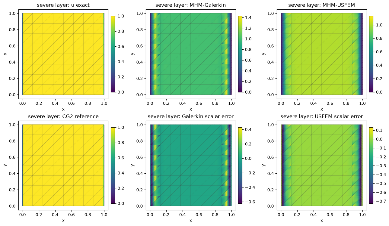
MHM-Galerkin overshoot = 0.4291224985130555 maximum nodal error = 0.46175828742208314 scalar L2 = 0.16028915457590862
MHM-USFEM overshoot = 0.13255967904081012 maximum nodal error = 0.17865926802559684 scalar L2 = 0.1993607741408251
7. Refine the local and trace spaces together
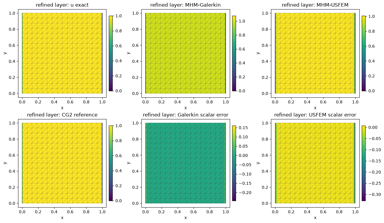
Keep P1 local polynomials and P0 on each face segment, but use four equal segments per macroface and eight local subdivisions. The eight-subdivision mesh is one red refinement of the matching four-subdivision mesh. We vary macro divisions through \(n=4,8,16\) for \(\epsilon=10^{-5}\) and also compute \(\epsilon=10^{-3}\) at \(n=16\) for the profile comparison.
The finest case has 512 macrotriangles and four P0 segments per face, as reported for the paper's analytical comparison. The paper states \(\bar H=H/4\) and \(h=\bar H\), but does not specify the historical matching triangulation and connectivity sufficiently to recover the local meshes. Our uniform red-refined realization is declared here. Moreover, the paper's continuous hybrid formulation imposes Dirichlet trace moments weakly; this tutorial imposes the exterior data strongly on local nodes. These are material differences when interpreting the discrete results. We compare the same analytical PDE and an admissible discretization; we do not claim a matched reproduction of Fig. 2.
The global equation is still the sum of local scalar-trace balances. Only the geometry and the number of face segments change below; the UFL forms, stabilization sign, source and boundary convention remain those already defined.
resolved_cases, resolved_rows = {}, []
FACE_SUBDIVISIONS, RESOLVED_LOCAL_SUBDIVISIONS = 4, 8
RESOLVED_LEVELS = {1e-5: (4, 8, 16)}
RESOLVED_LEVELS.setdefault(EPSILON, (16,))
for epsilon, resolutions in RESOLVED_LEVELS.items():
    for n in resolutions:
        for method, stabilized in METHODS:
            case, row, archive = measure_case(
                *solve_rad_case(
                    n,
                    epsilon,
                    stabilized,
                    face_subdivisions=FACE_SUBDIVISIONS,
                    local_subdivisions=RESOLVED_LOCAL_SUBDIVISIONS,
                ),
                ReactionLayer(epsilon),
                order=ERROR_ORDER,
                name=f"rad-resolved-eps{epsilon:g}-n{n}-{method.lower()}",
                epsilon=epsilon,
                method=method,
                n=n,
                H=1 / n,
                face_subdivisions=FACE_SUBDIVISIONS,
                local_subdivisions=RESOLVED_LOCAL_SUBDIVISIONS,
            )
            row["overshoot"] = max(0.0, row["nodal_maximum"] - 1)
            resolved_cases[epsilon, n, method] = case
            resolved_rows.append(row)
            state_archives.append(archive)
            print("Refined P1/P0", epsilon, n, method, row)
resolved_rows
Refined P1/P0 1e-05 4 MHM-Galerkin {'macro_cells': 32, 'fine_cells': 2048, 'trace_dofs': 224, 'residual': 3.582091155950077e-18, 'scalar_l2': 0.10038241445937039, 'flux_l2': 0.00016200323188130994, 'gradient_l2': 16.200323188130994, 'scalar_relative_l2': 0.10086198497393516, 'nodal_error': 0.3972480272375427, 'nodal_minimum': 0.0, 'nodal_maximum': 1.3971969472457781, 'epsilon': 1e-05, 'method': 'MHM-Galerkin', 'n': 4, 'H': 0.25, 'face_subdivisions': 4, 'local_subdivisions': 8, 'overshoot': 0.39719694724577814}
Refined P1/P0 1e-05 4 MHM-USFEM {'macro_cells': 32, 'fine_cells': 2048, 'trace_dofs': 224, 'residual': 5.996360824405177e-18, 'scalar_l2': 0.12651669686326633, 'flux_l2': 0.0001594287090734297, 'gradient_l2': 15.942870907342968, 'scalar_relative_l2': 0.12712112222743516, 'nodal_error': 0.1747988228416666, 'nodal_minimum': 0.0, 'nodal_maximum': 1.0203970217061842, 'epsilon': 1e-05, 'method': 'MHM-USFEM', 'n': 4, 'H': 0.25, 'face_subdivisions': 4, 'local_subdivisions': 8, 'overshoot': 0.020397021706184182}
Refined P1/P0 1e-05 8 MHM-Galerkin {'macro_cells': 128, 'fine_cells': 8192, 'trace_dofs': 832, 'residual': 1.647047208981743e-18, 'scalar_l2': 0.05166215678890528, 'flux_l2': 0.0001414541127895522, 'gradient_l2': 14.145411278955219, 'scalar_relative_l2': 0.051908969412891415, 'nodal_error': 0.3042539477792454, 'nodal_minimum': 0.0, 'nodal_maximum': 1.2971069210013073, 'epsilon': 1e-05, 'method': 'MHM-Galerkin', 'n': 8, 'H': 0.125, 'face_subdivisions': 4, 'local_subdivisions': 8, 'overshoot': 0.2971069210013073}
Refined P1/P0 1e-05 8 MHM-USFEM {'macro_cells': 128, 'fine_cells': 8192, 'trace_dofs': 832, 'residual': 3.602925898094949e-18, 'scalar_l2': 0.0718478396324243, 'flux_l2': 0.00013951315234044713, 'gradient_l2': 13.951315234044712, 'scalar_relative_l2': 0.07219108805505349, 'nodal_error': 0.18175214271977902, 'nodal_minimum': 0.0, 'nodal_maximum': 1.0156894150245483, 'epsilon': 1e-05, 'method': 'MHM-USFEM', 'n': 8, 'H': 0.125, 'face_subdivisions': 4, 'local_subdivisions': 8, 'overshoot': 0.015689415024548348}
Refined P1/P0 1e-05 16 MHM-Galerkin {'macro_cells': 512, 'fine_cells': 32768, 'trace_dofs': 3200, 'residual': 1.4601526170143782e-18, 'scalar_l2': 0.020178636803276615, 'flux_l2': 0.00010181469397222876, 'gradient_l2': 10.181469397222875, 'scalar_relative_l2': 0.020275038939916595, 'nodal_error': 0.16048431096663485, 'nodal_minimum': 0.0, 'nodal_maximum': 1.0759442211988917, 'epsilon': 1e-05, 'method': 'MHM-Galerkin', 'n': 16, 'H': 0.0625, 'face_subdivisions': 4, 'local_subdivisions': 8, 'overshoot': 0.07594422119889166}
Refined P1/P0 1e-05 16 MHM-USFEM {'macro_cells': 512, 'fine_cells': 32768, 'trace_dofs': 3200, 'residual': 3.344955980707496e-18, 'scalar_l2': 0.033115431616295654, 'flux_l2': 0.00010318176578351813, 'gradient_l2': 10.318176578351812, 'scalar_relative_l2': 0.03327363845626651, 'nodal_error': 0.1530380547529956, 'nodal_minimum': 0.0, 'nodal_maximum': 1.0068824167868782, 'epsilon': 1e-05, 'method': 'MHM-USFEM', 'n': 16, 'H': 0.0625, 'face_subdivisions': 4, 'local_subdivisions': 8, 'overshoot': 0.006882416786878176}
Refined P1/P0 0.001 16 MHM-Galerkin {'macro_cells': 512, 'fine_cells': 32768, 'trace_dofs': 3200, 'residual': 2.3064649475921167e-17, 'scalar_l2': 0.0008317865677838922, 'flux_l2': 0.0004019769798175291, 'gradient_l2': 0.4019769798175291, 'scalar_relative_l2': 0.0008742910293675748, 'nodal_error': 0.006999393894721817, 'nodal_minimum': 0.0, 'nodal_maximum': 0.9999997474222397, 'epsilon': 0.001, 'method': 'MHM-Galerkin', 'n': 16, 'H': 0.0625, 'face_subdivisions': 4, 'local_subdivisions': 8, 'overshoot': 0.0}
Refined P1/P0 0.001 16 MHM-USFEM {'macro_cells': 512, 'fine_cells': 32768, 'trace_dofs': 3200, 'residual': 2.4620553040580394e-17, 'scalar_l2': 0.0012263474872157788, 'flux_l2': 0.00040196928701191604, 'gradient_l2': 0.40196928701191603, 'scalar_relative_l2': 0.001289014091459563, 'nodal_error': 0.0055887100964260306, 'nodal_minimum': 0.0, 'nodal_maximum': 0.999999725960371, 'epsilon': 0.001, 'method': 'MHM-USFEM', 'n': 16, 'H': 0.0625, 'face_subdivisions': 4, 'local_subdivisions': 8, 'overshoot': 0.0}
Numerical output and provenance
[{'macro_cells': 32,
  'fine_cells': 2048,
  'trace_dofs': 224,
  'residual': 3.582091155950077e-18,
  'scalar_l2': 0.10038241445937039,
  'flux_l2': 0.00016200323188130994,
  'gradient_l2': 16.200323188130994,
  'scalar_relative_l2': 0.10086198497393516,
  'nodal_error': 0.3972480272375427,
  'nodal_minimum': 0.0,
  'nodal_maximum': 1.3971969472457781,
  'epsilon': 1e-05,
  'method': 'MHM-Galerkin',
  'n': 4,
  'H': 0.25,
  'face_subdivisions': 4,
  'local_subdivisions': 8,
  'overshoot': 0.39719694724577814},
 {'macro_cells': 32,
  'fine_cells': 2048,
  'trace_dofs': 224,
  'residual': 5.996360824405177e-18,
  'scalar_l2': 0.12651669686326633,
  'flux_l2': 0.0001594287090734297,
  'gradient_l2': 15.942870907342968,
  'scalar_relative_l2': 0.12712112222743516,
  'nodal_error': 0.1747988228416666,
  'nodal_minimum': 0.0,
  'nodal_maximum': 1.0203970217061842,
  'epsilon': 1e-05,
  'method': 'MHM-USFEM',
  'n': 4,
  'H': 0.25,
  'face_subdivisions': 4,
  'local_subdivisions': 8,
  'overshoot': 0.020397021706184182},
 {'macro_cells': 128,
  'fine_cells': 8192,
  'trace_dofs': 832,
  'residual': 1.647047208981743e-18,
  'scalar_l2': 0.05166215678890528,
  'flux_l2': 0.0001414541127895522,
  'gradient_l2': 14.145411278955219,
  'scalar_relative_l2': 0.051908969412891415,
  'nodal_error': 0.3042539477792454,
  'nodal_minimum': 0.0,
  'nodal_maximum': 1.2971069210013073,
  'epsilon': 1e-05,
  'method': 'MHM-Galerkin',
  'n': 8,
  'H': 0.125,
  'face_subdivisions': 4,
  'local_subdivisions': 8,
  'overshoot': 0.2971069210013073},
 {'macro_cells': 128,
  'fine_cells': 8192,
  'trace_dofs': 832,
  'residual': 3.602925898094949e-18,
  'scalar_l2': 0.0718478396324243,
  'flux_l2': 0.00013951315234044713,
  'gradient_l2': 13.951315234044712,
  'scalar_relative_l2': 0.07219108805505349,
  'nodal_error': 0.18175214271977902,
  'nodal_minimum': 0.0,
  'nodal_maximum': 1.0156894150245483,
  'epsilon': 1e-05,
  'method': 'MHM-USFEM',
  'n': 8,
  'H': 0.125,
  'face_subdivisions': 4,
  'local_subdivisions': 8,
  'overshoot': 0.015689415024548348},
 {'macro_cells': 512,
  'fine_cells': 32768,
  'trace_dofs': 3200,
  'residual': 1.4601526170143782e-18,
  'scalar_l2': 0.020178636803276615,
  'flux_l2': 0.00010181469397222876,
  'gradient_l2': 10.181469397222875,
  'scalar_relative_l2': 0.020275038939916595,
  'nodal_error': 0.16048431096663485,
  'nodal_minimum': 0.0,
  'nodal_maximum': 1.0759442211988917,
  'epsilon': 1e-05,
  'method': 'MHM-Galerkin',
  'n': 16,
  'H': 0.0625,
  'face_subdivisions': 4,
  'local_subdivisions': 8,
  'overshoot': 0.07594422119889166},
 {'macro_cells': 512,
  'fine_cells': 32768,
  'trace_dofs': 3200,
  'residual': 3.344955980707496e-18,
  'scalar_l2': 0.033115431616295654,
  'flux_l2': 0.00010318176578351813,
  'gradient_l2': 10.318176578351812,
  'scalar_relative_l2': 0.03327363845626651,
  'nodal_error': 0.1530380547529956,
  'nodal_minimum': 0.0,
  'nodal_maximum': 1.0068824167868782,
  'epsilon': 1e-05,
  'method': 'MHM-USFEM',
  'n': 16,
  'H': 0.0625,
  'face_subdivisions': 4,
  'local_subdivisions': 8,
  'overshoot': 0.006882416786878176},
 {'macro_cells': 512,
  'fine_cells': 32768,
  'trace_dofs': 3200,
  'residual': 2.3064649475921167e-17,
  'scalar_l2': 0.0008317865677838922,
  'flux_l2': 0.0004019769798175291,
  'gradient_l2': 0.4019769798175291,
  'scalar_relative_l2': 0.0008742910293675748,
  'nodal_error': 0.006999393894721817,
  'nodal_minimum': 0.0,
  'nodal_maximum': 0.9999997474222397,
  'epsilon': 0.001,
  'method': 'MHM-Galerkin',
  'n': 16,
  'H': 0.0625,
  'face_subdivisions': 4,
  'local_subdivisions': 8,
  'overshoot': 0.0},
 {'macro_cells': 512,
  'fine_cells': 32768,
  'trace_dofs': 3200,
  'residual': 2.4620553040580394e-17,
  'scalar_l2': 0.0012263474872157788,
  'flux_l2': 0.00040196928701191604,
  'gradient_l2': 0.40196928701191603,
  'scalar_relative_l2': 0.001289014091459563,
  'nodal_error': 0.0055887100964260306,
  'nodal_minimum': 0.0,
  'nodal_maximum': 0.999999725960371,
  'epsilon': 0.001,
  'method': 'MHM-USFEM',
  'n': 16,
  'H': 0.0625,
  'face_subdivisions': 4,
  'local_subdivisions': 8,
  'overshoot': 0.0}]
Inspect the refined physical fields and measured rates
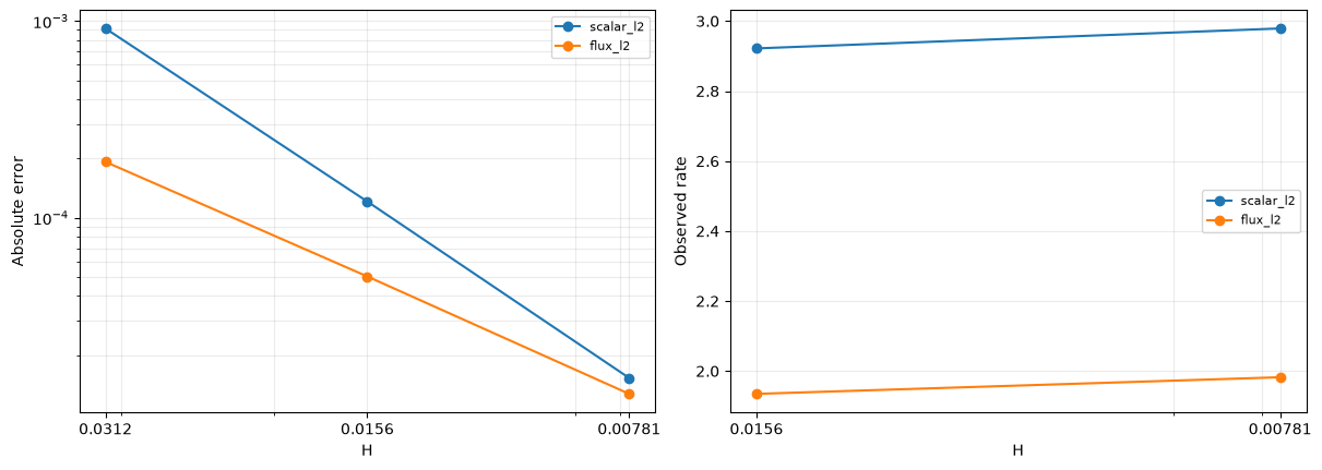
The following severe-layer panels use the finest declared P1/P0 family. They show both methods, their scalar errors and the independently refined CG2 baseline. Every panel overlays the actual 512-triangle macro mesh. The convergence figure reports observed scalar and physical-flux errors and slopes; no smooth-problem rate is transferred to this singularly perturbed case.
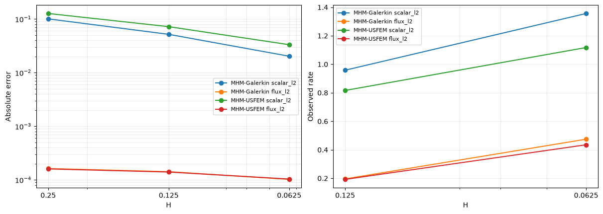
MHM-Galerkin scalar_l2 rates: [0.95833 1.35628]
MHM-Galerkin flux_l2 rates: [0.19569 0.47439]
MHM-USFEM scalar_l2 rates: [0.81631 1.11744]
MHM-USFEM flux_l2 rates: [0.19251 0.43521]
Verify physical integration at both resolution extremes
The severe coarse control uses Duffy rules with 40 and 48 Gaussian points per coordinate. Both finest refined methods use 24 and 32. These comparisons verify the reported scalar and raw physical-flux norms; an algebraic residual is recorded separately. Each solved state also archives its executed local basis and passes replay with one and two BLAS threads.
quadrature_controls: list[dict[str, Any]] = []
for family, orders in (("underresolved", (40, 48)), ("refined", (24, 32))):
    for method in ("MHM-Galerkin", "MHM-USFEM"):
        if family == "underresolved":
            meshes, fields = challenging[1e-5, method]
            measured = next(
                row for row in sweep if row["epsilon"] == 1e-5 and row["method"] == method
            )
        else:
            meshes, fields = resolved_cases[1e-5, 16, method][2:]
            measured = next(
                row
                for row in resolved_rows
                if row["epsilon"] == 1e-5 and row["n"] == 16 and row["method"] == method
            )
        higher = scalar_error_norms(
            meshes,
            fields,
            1,
            ReactionLayer(1e-5).value,
            ReactionLayer(1e-5).gradient,
            1e-5,
            order=orders[1],
        )
        norms = ("scalar_l2", "flux_l2")
        np.testing.assert_allclose(
            [higher[norm] for norm in norms],
            [measured[norm] for norm in norms],
            rtol=1e-8,
        )
        quadrature_controls.append(
            dict(
                family=family,
                method=method,
                epsilon=1e-5,
                orders=list(orders),
                norms={norm: [measured[norm], higher[norm]] for norm in norms},
            )
        )
quadrature_controls
[{'family': 'underresolved',
  'method': 'MHM-Galerkin',
  'epsilon': 1e-05,
  'orders': [40, 48],
  'norms': {'scalar_l2': [0.16028915457590862, 0.16028915457590864],
   'flux_l2': [0.00017088075366392442, 0.00017088075366392474]}},
 {'family': 'underresolved',
  'method': 'MHM-USFEM',
  'epsilon': 1e-05,
  'orders': [40, 48],
  'norms': {'scalar_l2': [0.1993607741408251, 0.19936077414082506],
   'flux_l2': [0.0001690370709830444, 0.00016903707098304475]}},
 {'family': 'refined',
  'method': 'MHM-Galerkin',
  'epsilon': 1e-05,
  'orders': [24, 32],
  'norms': {'scalar_l2': [0.020178636803276615, 0.020178636803276587],
   'flux_l2': [0.00010181469397222876, 0.00010181469397222887]}},
 {'family': 'refined',
  'method': 'MHM-USFEM',
  'epsilon': 1e-05,
  'orders': [24, 32],
  'norms': {'scalar_l2': [0.033115431616295654, 0.033115431616295626],
   'flux_l2': [0.00010318176578351813, 0.00010318176578351829]}}]
8. Compare coarse and refined one-sided profiles
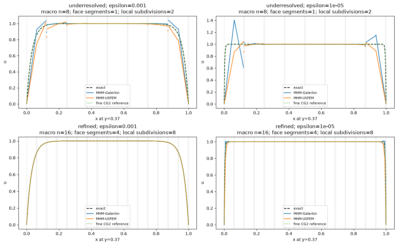
The top row preserves the \(n=8\), unsplit-face, two-local-subdivision control. The bottom row uses \(n=16\), four P0 segments per face and eight local subdivisions. Each panel includes the exact field and its corresponding fine CG2 reference. These meshes remain much smaller in the global multiscale solve than the reference mesh.
Horizontal profiles retain a separate segment for each incident macrocell. Vertical markers identify actual macroface crossings; neighboring endpoint values are evaluated independently instead of being averaged. Profiles need not agree pointwise across a macroface because the global equations enforce the declared trace moments.
For the coarse P1/P0 control at \(\epsilon=10^{-5}\), MHM-USFEM has smaller overshoot and maximum nodal error than MHM-Galerkin, but a larger scalar \(L^2\) error. At \(\epsilon=10^{-3}\), its maximum nodal error is larger.
provenance = execution_provenance(
    "notebooks/introduction/mhm_usfem_rad.ipynb",
    root=ROOT,
    execution={
        "policy": RAD_POLICY,
        "parallel_backend": RAD_EXECUTION.backend,
        "automatic_process_configuration": "at least 512 macroelements, 8 local subdivisions and 4 face segments",
        "workers": RAD_EXECUTION.effective_workers,
        "native_threads": RAD_EXECUTION.native_threads,
        "pipeline": RAD_EXECUTION.pipeline,
        "pending_bound": RAD_EXECUTION.effective_batch_size,
        "workers_capped_to_macroelement_count": True,
        "provider_source_sha256": RAD_PROVIDER_SOURCE_SHA256,
        "jit_cache": "notebook-owned temporary directory; serial two-orientation warm-up",
    },
    literature_comparison="same analytical PDE; declared SW-NE topology and strong exterior Dirichlet data; historical matching local triangulation/connectivity is unresolved; no matched-figure reproduction",
)
plot_rad_profiles(
    macro,
    challenging,
    resolved_cases,
    references,
    ReactionLayer,
    epsilon_primary=EPSILON,
    underresolved_subdivisions=LOCAL_SUBDIVISIONS,
    face_subdivisions=FACE_SUBDIVISIONS,
    refined_subdivisions=RESOLVED_LOCAL_SUBDIVISIONS,
    reports=REPORTS,
)
_ = (REPORTS / "mhm-usfem-rad.json").write_text(
    json.dumps(
        {
            "problem": "CILAMCE 2025 section 4.1 analytical reaction layer",
            "source_url": "https://doi.org/10.55592/cilamce2025.v5i.14270",
            "epsilon": EPSILON,
            "local_degree": 1,
            "trace_degree": 0,
            "local_subdivisions": LOCAL_SUBDIVISIONS,
            "local_ufl_quadrature_degree": LOCAL_QUADRATURE_DEGREE,
            "operator_check_duffy_order": OPERATOR_CHECK_ORDER,
            "reference_backend": f"DOLFINx {dolfinx.__version__}; independent CG2 UFL",
            "boundary": "strong u=0 vertical, zero physical flux horizontal",
            "convergence": rows,
            "reference_refinement": reference_rows,
            "provenance": provenance,
            "state_archives": state_archives,
            "reaction_sweep": sweep,
            "underresolved_configuration": {
                "macro_divisions": 8,
                "face_subdivisions": 1,
                "local_subdivisions": LOCAL_SUBDIVISIONS,
                "role": "fixed-space resolution control; stabilization has no nodal-bound guarantee",
            },
            "refined_convergence": resolved_rows,
            "refined_configuration": {
                "face_subdivisions": 4,
                "local_subdivisions": 8,
                "compatibility": f"P1/P0; face subdivisions={FACE_SUBDIVISIONS}, local subdivisions={RESOLVED_LOCAL_SUBDIVISIONS}",
                "boundary_variant": "strong exterior nodal Dirichlet data; continuous paper hybridization is weak",
                "literature_status": "same PDE and declared admissible realization, not matched historical Fig2",
                "unresolved_paper_input": "matching local triangulation and macro connectivity for Fig2",
            },
            "quadrature_controls": quadrature_controls,
        },
        indent=2,
    )
    + "\n"
)

# All local assembly is complete; release the notebook-owned compiler cache.
sys.path.remove(RAD_JIT_CACHE.name)
sys.modules.pop(RAD_WORKER_MODULE_NAME, None)
RAD_JIT_CACHE.cleanup()
9. Qualify smooth convergence separately from the sharp layer
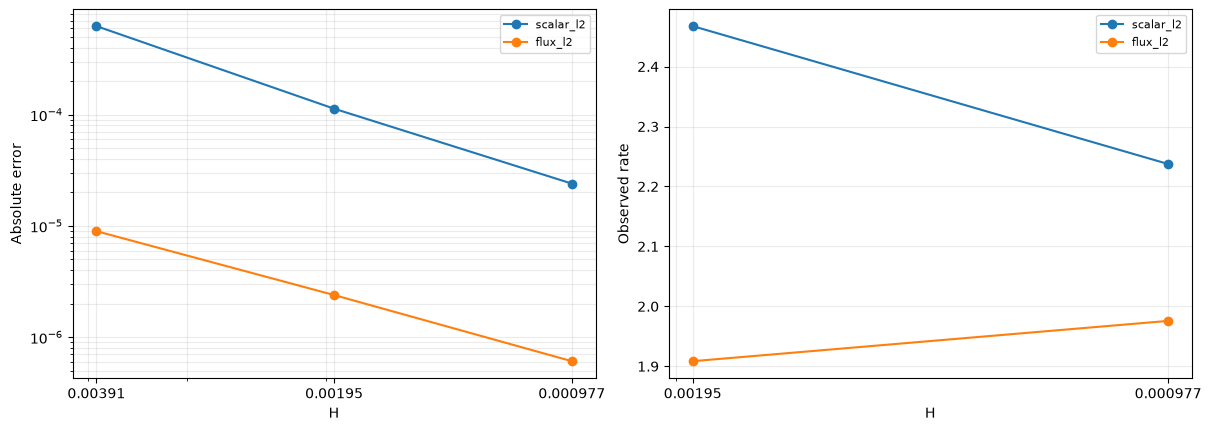
The layer experiments above test practical behavior as diffusion decreases. An underresolved singular perturbation does not qualify a smooth asymptotic rate. For a separate control, use the analytical problem of section 4.1 in Martins, Pacazuca and Valentin (2025), with \(\epsilon=\sigma=1\) and \(f=1\):
Vertical exterior sides impose zero scalar values; horizontal sides impose zero outward physical flux. Local P1 scalar uses one red refinement and the skeleton uses P0 traces. This is the admissible \(k=\ell+1\) refined alternative of Theorem 1. Preserve the negative residual pairing and its independently derived stabilized source. Refine the macro diameter through \(n=2,4,8,16,32\), with two local subdivisions at every level.
Theorem 1, estimate (21), contains skeletal and local approximation terms and an additional sum depending on the fine-cell Péclet numbers. Figure 1 supplies the smooth numerical reference orders: one in H1 and two in scalar L2. The theorem does not state a separate scalar L2 estimate. These observations do not supply diffusion-uniform rates for the sharp layers above; the layer plots and their physical errors answer a separate resolution question.
Recompute every measured order
For successive physical errors \(E_{i-1},E_i\) at the actual macro diameters, compute
The cell reads the attributed numerical record, displays every measured level and recomputes its orders. It does not execute a PDE acquisition. The fitted terminal slope uses the final four levels and their three intervals. For each declared target \(q\), the amplitude ratio is the maximum divided by the minimum of \(E/H^q\) over those same levels. A value near one indicates stabilization of the compensated error; an observed L2 order is kept separate from a proved energy estimate.
import json
import matplotlib.pyplot as plt
from IPython.display import Markdown, display
from examples.tutorial_convergence import refinement_series, asymptotic_summary, plot_method_series
refinement_record = ROOT / 'examples/results/unusual/analytical.json'
refinement_data = json.loads(refinement_record.read_text(encoding='utf-8'))
refinement_rows = [dict(H=2 ** 0.5 / refinement_row['n'], **refinement_row) for refinement_row in refinement_data['rows'] if refinement_row['case'] == 'smooth' and refinement_row['method'] == 'unusual']
refinement_error_keys = {'scalar L2': 'scalar_l2', 'broken gradient L2': 'gradient_l2'}
refinement_targets = {'broken gradient L2': 1.0}
refinement_rows = sorted(refinement_rows, key=lambda refinement_row: refinement_row['H'], reverse=True)
refinement_sizes = np.asarray([refinement_row['H'] for refinement_row in refinement_rows])
refinement_field_errors = {refinement_field: np.asarray([refinement_row[refinement_key] for refinement_row in refinement_rows]) for refinement_field, refinement_key in refinement_error_keys.items()}
refinement_orders = {refinement_field: np.log(refinement_values[:-1] / refinement_values[1:]) / np.log(refinement_sizes[:-1] / refinement_sizes[1:]) for refinement_field, refinement_values in refinement_field_errors.items()}
refinement_header = ['Refinement size'] + [refinement_column for refinement_field in refinement_error_keys for refinement_column in (refinement_field, 'Order')]
refinement_lines = [' | '.join(refinement_header), ' | '.join(['---'] * len(refinement_header))]
for refinement_index, refinement_size in enumerate(refinement_sizes):
    refinement_values = [f'{refinement_size:.6g}']
    for refinement_field in refinement_error_keys:
        refinement_values.extend([f'{refinement_field_errors[refinement_field][refinement_index]:.6e}', '—' if refinement_index == 0 else f'{refinement_orders[refinement_field][refinement_index - 1]:.3f}'])
    refinement_lines.append(' | '.join(refinement_values))
display(Markdown('\n'.join(refinement_lines)))
refinement_series_data = refinement_series(refinement_record, refinement_rows, 'H', refinement_error_keys, refinement_targets, method='mhm-usfem', spaces='P1/r2 locals; P0 trace; epsilon=sigma=1; negative residual pairing', rate_provenance='Martins, Pacazuca and Valentin (2025), Theorem 1: admissible reaction-diffusion energy bound with local Peclet factor; Figure 1 smooth numerical orders', root=ROOT)
print({'record': refinement_series_data['record'], 'sha256': refinement_series_data['sha256']})
for refinement_field, refinement_summary in asymptotic_summary(refinement_series_data).items():
    print(refinement_field, {'last_three_orders': [round(refinement_order, 3) for refinement_order in refinement_summary['orders']], 'fitted_order': round(refinement_summary['fitted_order'], 3), 'target': refinement_summary['target'], 'normalized_amplitude_ratio': refinement_summary.get('amplitude_ratio')})
plot_method_series(refinement_series_data)
plt.show()
| Refinement size | scalar L2 | Order | broken gradient L2 | Order |
|---|---|---|---|---|
| 0.707107 | 1.965642e-02 | — | 1.211875e-01 | — |
| 0.353553 | 5.527338e-03 | 1.830 | 6.541841e-02 | 0.889 |
| 0.176777 | 1.457502e-03 | 1.923 | 3.387681e-02 | 0.949 |
| 0.0883883 | 3.746517e-04 | 1.960 | 1.723394e-02 | 0.975 |
| 0.0441942 | 9.503769e-05 | 1.979 | 8.691650e-03 | 0.988 |
{'record': 'examples/results/unusual/analytical.json', 'sha256': 'e83d4dc1617b3ab8473dac0135fef861797fa057436f81a76718b70f45ab5c61'}
scalar L2 {'last_three_orders': [1.923, 1.96, 1.979], 'fitted_order': 1.955, 'target': None, 'normalized_amplitude_ratio': None}
broken gradient L2 {'last_three_orders': [0.949, 0.975, 0.988], 'fitted_order': 0.971, 'target': 1.0, 'normalized_amplitude_ratio': 1.0628994737060553}
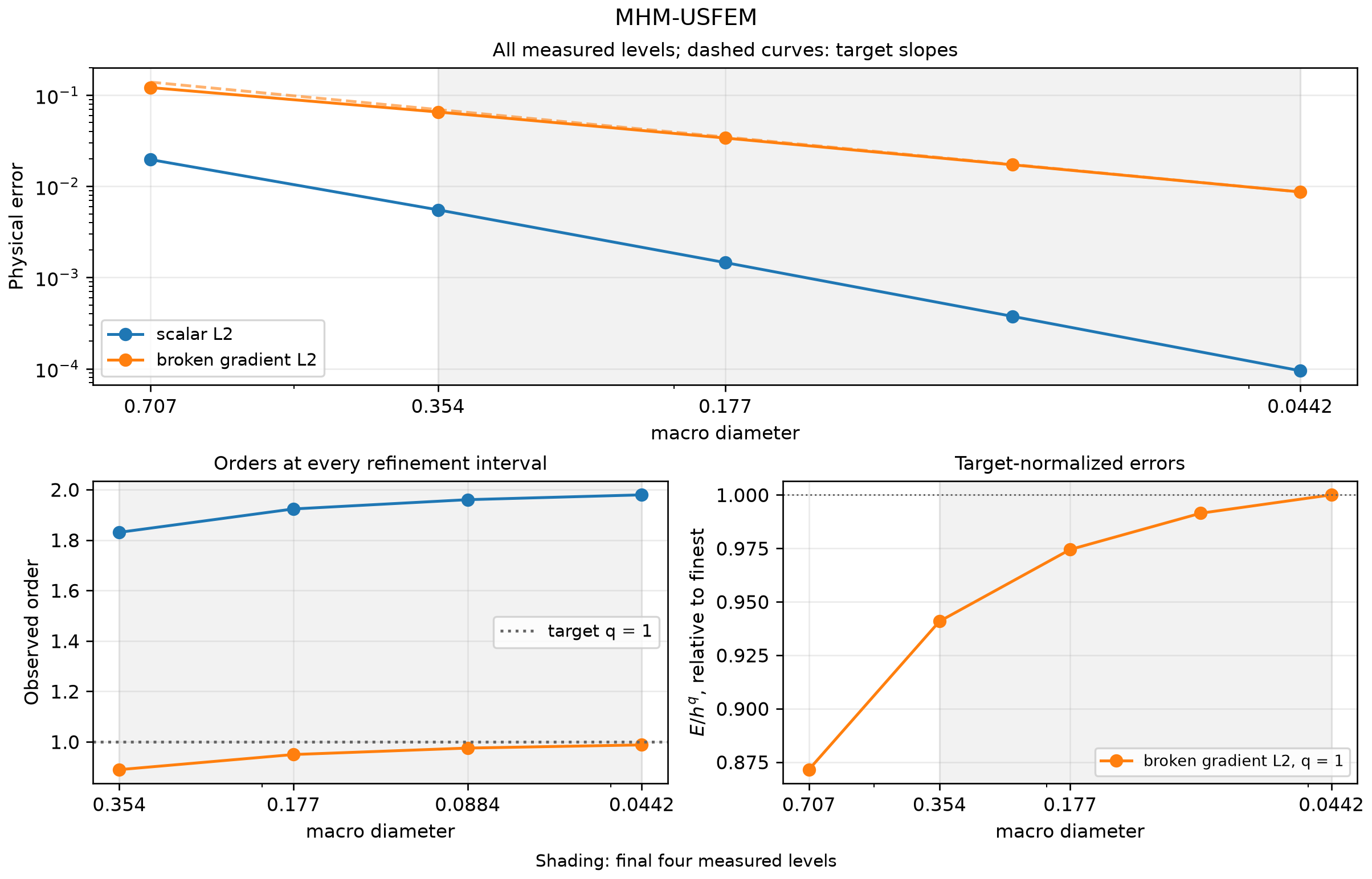
Download the figure as SVG or PDF. Shading covers the same final four levels in every panel; dashed curves are target powers anchored to the finest measured error.
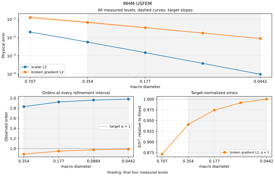
The smooth convergence figure uses the attributed numerical record (SHA256 e83d4dc1617b3ab8473dac0135fef861797fa057436f81a76718b70f45ab5c61). The shared rate notebook compares the method sequences.
Reproduce this tutorial
View the source notebook or download the notebook, then open it:
The first cell downloads a SHA256-verified companion containing inspectable support files. Downloading does not execute them. Native UFL forms require the compatible backend described in the installation guide.
For batch execution, extract the same companion, change to its workspace and run:
The runner uses the active interpreter and writes an executed copy and receipt under build/notebooks/introduction/. Larger field archives have documented downloads.
Figures and outputs of sections 1–8 retain notebook SHA256 4e04e823bd700e3108ff564015f0a611ceb9524697759692cd4238911541cbb6 in the publication manifest. The smooth convergence figure and tables use the separate numerical records cited in section 9. Running the current source produces a receipt for its actual notebook, support files and environment.
References
-
Larissa Martins, Juan F. Pacazuca, and Frédéric Valentin (2025). A Multiscale Hybrid-Mixed Method with Local Stabilization. Proceedings of the Ibero-Latin American Congress on Computational Methods in Engineering, CILAMCE 2025, volume 5, article 14270; published online 18 March 2026. DOI: 10.55592/cilamce2025.v5i.14270.
-
L. P. Franca and Frédéric Valentin (2000). On an improved unusual stabilized finite element method for the advective–reactive–diffusive equation. Computer Methods in Applied Mechanics and Engineering 190(13–14), 1785–1800. DOI: 10.1016/S0045-7825(00)00190-0.