Waves in a photonic device

An incident electromagnetic wave crosses a silica device containing fifteen circular inclusions. The material geometry redirects the wave; local DG electric and magnetic fields communicate through tangential macroface traces.

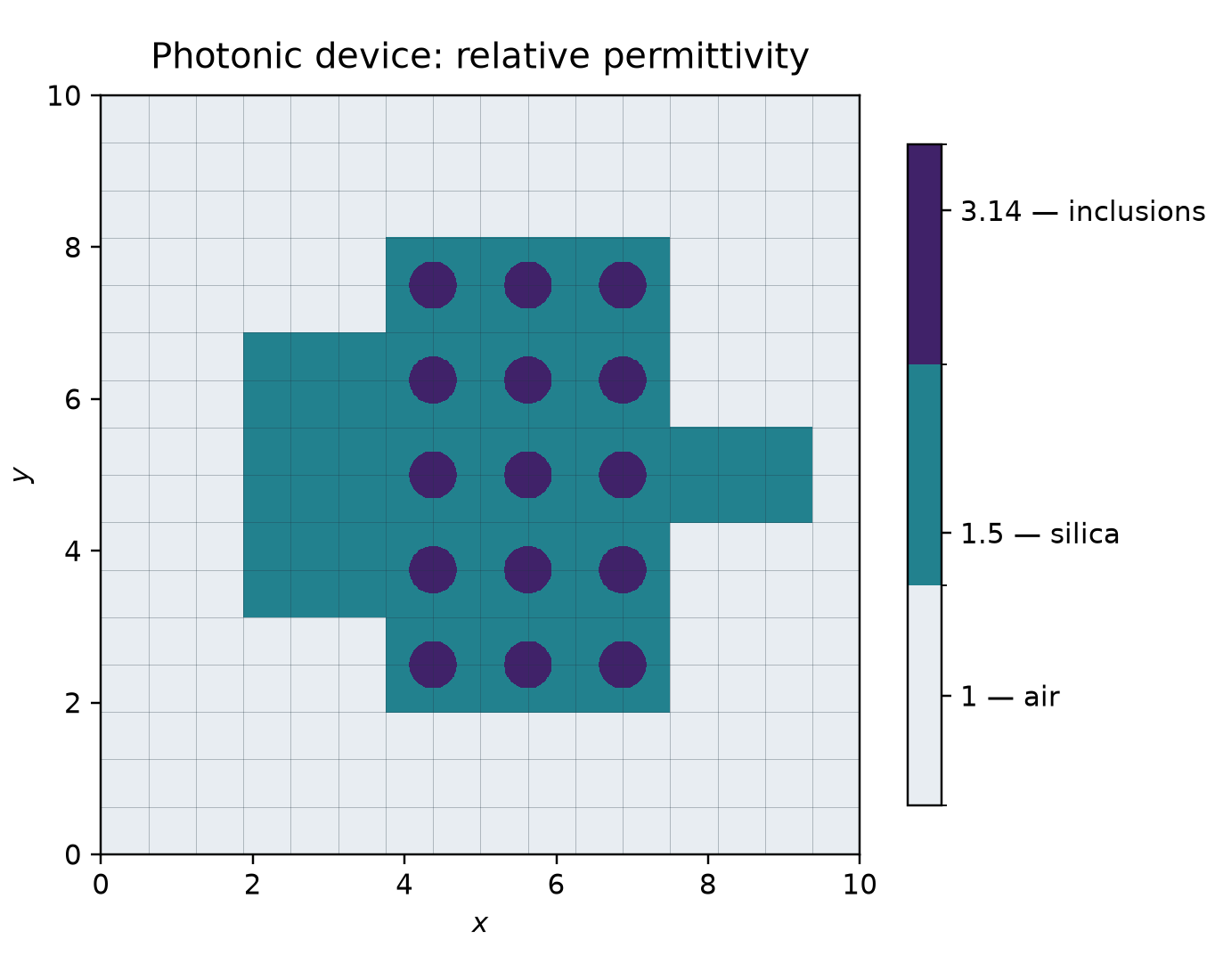
This figure shows the prescribed relative permittivity. Its three colors denote air, silica and inclusions. Computed electric and magnetic fields are reported in the complete result report.

Physical problem

The two-dimensional TM system on \(\Omega=(0,10)^2\) has electric component \(E_z\) and magnetic vector \(\boldsymbol H=(H_x,H_y)\):

\[ \begin{aligned} \epsilon\,\partial_t E_z-\operatorname{curl}\boldsymbol H&=0,\\ \mu\,\partial_t\boldsymbol H+\operatorname{curl}E_z&=0. \end{aligned} \]

Here \(\operatorname{curl}\boldsymbol H=\partial_xH_y-\partial_yH_x\) and \(\operatorname{curl}E_z=(\partial_yE_z,-\partial_xE_z)\). Magnetic permeability is one. Relative permittivity is 1 in air, 1.5 in silica and 3.14 in the circular inclusions; these are permittivities, not refractive indices to be squared.

The silica is the union of three rectangles: \([3.75,7.5]\times[1.875,8.125]\), \([1.875,3.75]\times[3.125,6.875]\) and \([7.5,9.375]\times[4.375,5.625]\). Inclusions have radius 0.3125 and centers

\[ \{4.375,5.625,6.875\}\times\{2.5,3.75,5,6.25,7.5\}. \]

Initial fields vanish. A causal unit-amplitude incident wave and absorbing boundary data are

\[ \begin{aligned} E_i(t,x,y)&=\mathbf1_{t\geq x}\sin(\pi(t-x)),\\ \boldsymbol H_i&=(0,-E_i),\\ E_z-(\boldsymbol H\times\boldsymbol n)&=(1-n_x)E_i. \end{aligned} \]

The publication supplies frequency and final time, but not a unique phase and turn-on convention. These declared data are identical in every comparison; they are not identified with an unspecified historical transient.

Multiscale formulation and implementation

The two acquired MHM configurations use \(16\times16\) macros with \(8\times8\) local DG \(Q_2\) cells, or \(8\times8\) macros with \(16\times16\) local cells. Both have \(128\times128\) fine quadrilaterals. Tangential \(P_1\) traces use one segment per local boundary edge. The macro time increment is 0.01.

For an electric kick of duration \(\tau\), midpoint electric field \(w\) and canonical trace \(\lambda=\boldsymbol H\times\boldsymbol n\) satisfy

\[ \begin{aligned} M_e w+\tfrac{\tau}{2}Q\lambda &=M_e E_{\rm old}+\tfrac{\tau}{2}(F-C^{\mathsf T}H),\\ -\sum_T Q_T^{\mathsf T}w_T+Z\lambda&=-b,\\ E_{\rm new}&=2w-E_{\rm old}. \end{aligned} \]

The first row is local; the second is the global tangential equation, including exterior impedance \(Z\) and boundary moments \(b\). With \(C=-\operatorname{curl}\), the magnetic update is the independent local mass problem \(M_hH_{\rm new}=M_hH_{\rm old}+\Delta t\,CE\).

The application passes the electric equation to the generic API:

return LocalEquations(
    a=local.electric_mass,
    L=local.electric_mass @ electric + duration / 2 * (source - local.curl.T @ magnetic),
    b=duration / 2 * local.coupling,
    c=-local.coupling.T,
    dofs=local.trace_dofs,
)

The Maxwell tutorial explains these providers and the global equation separately from the device. The application notebook specifies the material and transient, invokes the declared equations, and reads the archived componentwise comparisons.

Results and reproducibility

At matched staggered times \(t_E=11.315\) and \(t_H=11.31\), the two MHM configurations differ from the finest classical DG reference by 0.835% and 0.724% in combined unweighted physical L2 field norm. A coarse \(32\times32\) classical DG calculation differs by 13.01%.

The finest reference has \(1024\times1024\) DG \(Q_2\) cells and time step 0.00125. Separate reference spatial, temporal and material-quadrature controls give increments 0.127%, 0.080% and 0.035%, respectively. These numerical-reference increments quantify sensitivity; they are not rigorous bounds on its remaining error. The device baseline uses central DG. Its qualification does not include a separately refined conforming transient reference for these heterogeneous material and incident data.

The complete result report provides componentwise norms, physical times, reference controls and reproduction commands. The material figure is reproducible from the application's permittivity function; its plot record states source hashes and its material-only scope.

References

• Stéphane Lanteri, Diego Paredes, Claire Scheid and Frédéric Valentin (2018). The Multiscale Hybrid-Mixed method for the Maxwell Equations in Heterogeneous Media. DOI: 10.1137/16M110037X.