MsHHO: cell and face moments
Open the step-by-step notebook · Download notebook
Follow the numbered steps: state the variational problem, choose the local and trace spaces, declare the local and global equations, solve, and inspect the physical fields.
The main workflow is meshes → spaces → local equations → global balance → assemble → solve → fields and errors. MeshHierarchy associates macro and local meshes; bind_interface and LocalContext own supported numbering, geometric orientation and native coordinate conversions. The mathematical forms, physical trace meaning, local modes and gauge remain explicit in the cells below. Fully manual/custom spaces use the same numerical owners; see the custom-interface notebook.
We build a simple Multiscale Hybrid High-Order Darcy problem and explain every local and global block. All case definitions, equations, boundary conditions, reference solves, norms and plots are visible in this notebook. The weak operator is written in UFL. PyMHM provides generic compilation, trace pairings, constrained reconstruction and linear algebra.
The method family follows Chaumont-Frelet, Ern, Lemaire and Valentin (2022), sections 4–5. Their local spaces are defined by exactly solved PDEs. We use a finite local Galerkin realization on declared fine meshes. This original introductory problem is not a reproduction of an article figure or table.
The projected-source exact-local construction has the physical \(H(\mathrm{div})\) property of Lemma 4.2. Remark 5.3's reconstructed-source variant can lose that property even with exact local solves. The finite Galerkin flux must therefore be assessed in its actual source convention and local space; shared pressure moments alone do not give a conforming normal flux.
Run with the installed package in a writable directory and the compatible native DOLFINx/UFL backend:
Prerequisites: a weak Poisson formulation, basic NumPy and Jupyter. Cell-defined providers are used in serial execution; process workers require importable callables.
Field evaluation, norms, plots and executed-array archives use the importable supporting scalar helpers. The physical data and local/global variational equations remain explicit below.
The PyMHM distribution contains only the library. The first cell explicitly
downloads a checksum-verified companion archive and prepares the declared data
using its local Python helpers. You can inspect these support files in ROOT.
Complete studies and historical replay retain their existing opt-in flags.
from pathlib import Path
import os
import sys
from pymhm.io.workspace import workspace_from_archive

# Download verified support files; this operation does not execute them.
COMPANION_URL = "https://ipes-lncc.github.io/pymhm/downloads/c6b3e4e96bcbd504442e8fb9d7fc8f9474603b5609d123d79225f62d97167e2c/mshho_multiscale-companion.zip"
COMPANION_SHA256 = "c6b3e4e96bcbd504442e8fb9d7fc8f9474603b5609d123d79225f62d97167e2c"
WORKSPACE = Path(
    os.environ.get("PYMHM_WORKSPACE", Path.cwd() / ".pymhm-companions" / COMPANION_SHA256)
)
ROOT = workspace_from_archive(COMPANION_URL, sha256=COMPANION_SHA256, directory=WORKSPACE)
os.environ["PYMHM_WORKSPACE"] = str(ROOT)
if str(ROOT) not in sys.path:
    sys.path.insert(0, str(ROOT))

# Explicitly prepare declared data with the downloaded Python helpers.
from scripts.notebook_reproduction import notebook_workspace

ROOT = notebook_workspace("introduction/mshho_multiscale.ipynb", directory=ROOT)
root = ROOT
print("Workspace:", ROOT)


import numpy as np
import matplotlib.pyplot as plt
from typing import Any
from scipy import sparse
from threadpoolctl import threadpool_limits
from pymhm import Equation, LocalEquations, assemble
from pymhm import MeshHierarchy, LocalContext, bind_interface, bind_problem
from pymhm.core.equations import compile_form
from pymhm.fem.traces.interval import FaceSpace, SkeletonSpace
from examples.introduction.scalar import (
    plot_material,
    plot_reference_differences,
    plot_scalar_comparison,
    executed_array_digest,
    ScalarField,
    archive_cell,
    compare_scalar_fields,
    dirichlet_solve,
    native_scalar_space,
    save_scalar_report,
)
from pymhm.fem.scalar.triangle import nodal_space
from pymhm.meshes.triangle import TriangleMesh
from pymhm.backends.forms import assemble_pairing

plt.rcParams.update({"figure.dpi": 110, "font.size": 10})
from pymhm.core.moments import energy_reconstruction
1. Define the physical problem, material period and meshes
On \(\Omega=(0,1)^2\), solve
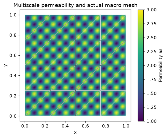
The bounds \(1\le a_\varepsilon\le3\) give uniform ellipticity. The coefficient period \(\varepsilon=1/8\) is physical data: eight material oscillations fit in each direction. The macro and local meshes are discretization choices. Our macro mesh has four squares per direction, split into 32 triangles; each macrocell contains material variation. Its independent local Galerkin problem uses 16 subdivisions per macroedge. The coarse unknowns are cell and face moments. Cell moments are eliminated locally, leaving a global system of face moments; the fine local fields resolve the coefficient variation.
TriangleMesh defines geometry. Below, we write and execute the form \(\int_K a_\varepsilon\nabla u\cdot\nabla v\) and load \(\int_K v\) in UFL before introducing optional assembly conveniences.
epsilon = 1 / 8


def permeability(points: np.ndarray) -> np.ndarray:
    """Evaluate aε I through its positive scalar factor, with ε=1/8."""
    phase = 2 * np.pi * points / epsilon
    return 2 + np.sin(phase[:, 0]) * np.sin(phase[:, 1])


macro = TriangleMesh.unit_square(4)
source = 1.0
local_refinement = 16
assembly_order = 8
print(
    {
        "macro_triangles": len(macro.cells),
        "epsilon": epsilon,
        "H_max": float(macro.lengths.max()),
        "h_max": float(macro.lengths.max() / local_refinement),
        "ellipticity_bounds": [1.0, 3.0],
        "source": source,
    }
)
{'macro_triangles': 32, 'epsilon': 0.125, 'H_max': 0.3535533905932738, 'h_max': 0.02209708691207961, 'ellipticity_bounds': [1.0, 3.0], 'source': 1.0}
2. The unknowns are pressure moments
Choose \(m=k_F=1\): three P1 volume moments per macrotriangle and two P1 moments per macroface. We store integrals rather than polynomial projection coefficients. The two coordinate systems are related by invertible polynomial mass matrices:
Here \(\widehat x,\widehat y\) are Cartesian coordinates scaled to the macrocell bounding box. They span P1 on each triangle. Both incident macrocells share \(z_F\); their complete fine nodal fields remain independent. Exterior face moments are zero by Dirichlet data.
SkeletonSpace numbers these face coordinates. Its name does not determine their physical meaning: these are pressure moments, not flux coefficients. Our local finite space is continuous P2; the moment constraints must be independent in that space.
local_degree = 2
skeleton = SkeletonSpace(macro, tuple(FaceSpace.uniform(1) for _ in macro.faces))
fixed = {int(dof): 0.0 for face in macro.boundary_faces for dof in skeleton.dofs(int(face))}
global_free_unknowns = skeleton.size - len(fixed)
print(
    {
        "face_moments_total": skeleton.size,
        "face_moments_free": global_free_unknowns,
        "cell_moments_per_macrocell": 3,
        "local_polynomial_degree": local_degree,
    }
)
{'face_moments_total': 112, 'face_moments_free': 80, 'cell_moments_per_macrocell': 3, 'local_polynomial_degree': 2}
3. Construct the local basis by constrained energy minimization
Let \(A_K\) be the fine stiffness and \(C_K\) the matrix of volume and face functionals. The reconstruction \(R_K\) gives the minimum-energy field with prescribed moments:
The Neumann stiffness has the constant kernel. Independent moments fix it; the stiffness must also be coercive on the moment-zero space. A small residual alone does not prove these properties.
The P1 cell tests are represented exactly at P2 nodes, so mass @ cell_tests integrates their volume moments. The face functionals are written directly as phi * v * ds with UFL. The value interface binding owns their geometry and numbering: pressure moments have no normal-incidence sign. The volume coefficients use the native space binding's executed nodal convention.
energy_reconstruction solves the generic \(A/C\) saddle above. It receives no physical-model or method selector. The constant source belongs to P1: in integral-moment coordinates the projected-source functional is simply \(z_{K,0}\), hence load \((1,0,0)\) on cell coordinates and zero on face coordinates.
Write the local differential operator in UFL
Define the trial pressure p and test pressure v on the local Pk space. The UFL expressions below are the executable weak form, mass pairing and source. Changing this expression defines a new local operator; the multiscale contracts do not select a physical model.
The small geometry adapter keeps the same fine triangles and equispaced nodal basis. It maps native coefficients by their physical coordinates; it contains no PDE. compile_form assembles the expressions and releases native assembly resources. The interface pairing is introduced separately, with its declared normal convention.
import basix.ufl
import ufl
from pymhm.backends.forms import assemble_pairing


def user_volume_forms(
    fine: TriangleMesh, degree: int, *, binding: Any = None
) -> tuple[Any, Any, np.ndarray]:
    """Execute the user-written weak operator, mass and source in the stated basis."""
    if binding is None:
        _, V, order = native_scalar_space(fine, degree)
    else:
        V, order = binding.space, binding.mapping
    p, v = ufl.TrialFunction(V), ufl.TestFunction(V)
    x = ufl.SpatialCoordinate(V.mesh)
    a_epsilon = 2 + ufl.sin(2 * np.pi * x[0] / epsilon) * ufl.sin(2 * np.pi * x[1] / epsilon)
    dx = ufl.Measure("dx", domain=V.mesh, metadata={"quadrature_degree": 2 * assembly_order})
    a = a_epsilon * ufl.inner(ufl.grad(p), ufl.grad(v)) * dx
    mass = p * v * dx
    L = source * v * dx
    A, M, F = compile_form(a), compile_form(mass), compile_form(L)
    return A[order][:, order].tocsc(), M[order][:, order].tocsc(), F[order]
first_fine = macro.submesh(0, local_refinement)
A_ufl, M_ufl, F_ufl = user_volume_forms(first_fine, local_degree)
print(
    {
        "operator": "user-written UFL",
        "local_nodal_unknowns": A_ufl.shape[0],
        "constant_kernel_relative": float(
            np.linalg.norm(A_ufl @ np.ones(A_ufl.shape[0])) / sparse.linalg.norm(A_ufl)
        ),
    }
)
form_equivalence = {}  # Filled by the optional convenience check at the end.
{'operator': 'user-written UFL', 'local_nodal_unknowns': 561, 'constant_kernel_relative': 3.6207041887734765e-16}
def local_moment_equations(local: LocalContext) -> LocalEquations:
    """Declare MsHHO P1 cell/face moments on a local conforming P2 space."""
    cell, fine = local.cell, local.mesh
    binding = local.native_space(
        basix.ufl.element(
            "Lagrange",
            "triangle",
            local_degree,
            lagrange_variant=basix.LagrangeVariant.equispaced,
        )
    )
    stiffness, mass, force = user_volume_forms(fine, local_degree, binding=binding)
    _, nodes = nodal_space(fine, local_degree)
    vertices = macro.points[macro.cells[cell]]
    scaled_xy = 2 * (nodes - vertices.min(axis=0)) / np.ptp(vertices, axis=0) - 1
    cell_tests = np.column_stack((np.ones(len(nodes)), scaled_xy))
    volume_moments = mass @ cell_tests
    v = ufl.TestFunction(binding.space)
    face_functionals = local.trace_pairings(lambda phi, ds: phi * v * ds)
    face_moments = assemble_pairing(face_functionals.forms, axis="columns")[binding.mapping]
    moments = np.column_stack((volume_moments, face_moments))
    reconstruction, energy = energy_reconstruction(stiffness, moments)

    # The declared source is constant. Since the first cell moment is
    # integral_K p, its load coordinate is source; all other coordinates vanish.
    moment_load = np.r_[source, np.zeros(moments.shape[1] - 1)]
    ncell = volume_moments.shape[1]
    return local.equations(
        a=energy[:ncell, :ncell],
        L=moment_load[:ncell],
        b=energy[:ncell, ncell:],
        c=energy[ncell:, :ncell],
        coordinates="global",
        d=energy[ncell:, ncell:],
        g=moment_load[ncell:],
        metadata={
            "mesh": fine,
            "R": reconstruction,
            "C": moments,
            "A": stiffness,
            "F": force,
            "energy": energy,
        },
    )
4. The global problem contains face moments
Partition \(E_K\) into cell (\(c\)) and face (\(F\)) blocks. The projected-source formulation becomes
These are exactly LocalEquations: a,L,b define the first equation; c,d,g contribute the second. assemble eliminates the three cell moments and adds shared face contributions.
Equation(0, zeros) supplies no additional global term. retained=0 retains no extra modes: the fine stiffness kernel has already been fixed in the constrained reconstruction, and cell moments are ordinary eliminated local unknowns. Prescribed exterior pressure moments remove the global pressure gauge.
After solving, solution.fields contains cell moments. Multiplying the complete local moment vector by the executed \(R_K\) recovers physical nodal pressure. The small field record below only associates coefficients with their declared mesh and Pk basis; it is not a solver.
hierarchy = MeshHierarchy(
    macro, tuple(macro.submesh(cell, local_refinement) for cell in range(len(macro.cells)))
)
problem = bind_problem(
    hierarchy,
    bind_interface(skeleton, convention="value"),
    local_moment_equations,
    global_equation=Equation(0, 0),
    retained=0,
    fixed=fixed,
)
with threadpool_limits(1):
    system = assemble(problem)
    solution = system.solve()

# solution.fields contains cell moments, not physical nodal pressures.
physical_fields = tuple(
    ScalarField(
        data["mesh"], local_degree, data["R"] @ np.r_[cell_moments, solution.local_trace(cell)]
    )
    for cell, (data, cell_moments) in enumerate(
        zip(system.local_metadata, solution.fields, strict=True)
    )
)
print(
    {
        "global_free_unknowns": global_free_unknowns,
        "global_residual": solution.residual,
        "local_nodal_unknowns_per_macrocell": len(physical_fields[0].values),
    }
)
{'global_free_unknowns': 80, 'global_residual': 7.994602283557082e-17, 'local_nodal_unknowns_per_macrocell': 561}
5. Check the kernel and the executed moment basis
Check \(A_K1=0\), \(C_K^TR_K=I\), and the moments of the recovered pressure. Full pressure may jump across a macroface; its P1 face moments agree.
The finite local Galerkin realization does not automatically inherit the ideal article space's \(H(\mathrm{div})\) flux property. We report the raw physical flux \(-a_\varepsilon\nabla p_h\) inside each fine element and do not assert fine-cell conservation.
Archive each executed \(R_K\) with its SHA256 digest and the complete moment vector. Field replay uses that same matrix; persisted moment coefficients must not be applied to a numerically changed basis.
The physical reconstruction reads solution.local_trace(cell): the bound space supplies the executed local face coefficients, including any declared basis changes. The value convention used here has no outward-normal sign. The method's reconstruction matrix remains an explicit part of its mathematical definition.
diagnostics = {
    "constant_kernel_relative": 0.0,
    "moment_identity_max": 0.0,
    "recovered_moment_max": 0.0,
}
basis_digests = []
archive = {"macro_points": macro.points, "macro_cells": macro.cells, "face_moments": solution.trace}
for cell, (data, field, cell_moments) in enumerate(
    zip(system.local_metadata, physical_fields, solution.fields, strict=True)
):
    A, C, R = data["A"], data["C"], data["R"]
    target = np.r_[cell_moments, solution.local_trace(cell)]
    diagnostics["constant_kernel_relative"] = max(
        diagnostics["constant_kernel_relative"],
        float(np.linalg.norm(A @ np.ones(A.shape[0])) / np.linalg.norm(A.data)),
    )
    diagnostics["moment_identity_max"] = max(
        diagnostics["moment_identity_max"],
        float(np.max(abs(C.T @ R - np.eye(C.shape[1])))),
    )
    diagnostics["recovered_moment_max"] = max(
        diagnostics["recovered_moment_max"],
        float(np.max(abs(C.T @ field.values - target))),
    )
    basis_digests.append(executed_array_digest(R))
    archive_cell(archive, cell, field, reconstruction=R, moments=C, moment_coordinates=target)
assert max(diagnostics.values()) < 1e-10
print(diagnostics)
{'constant_kernel_relative': 3.644021074115437e-16, 'moment_identity_max': 2.4424906541753444e-15, 'recovered_moment_max': 2.8189256484623115e-18}
6. A classical primal Galerkin baseline, with its own refinement check
On a fine globally conforming mesh, the baseline solves the same operator, material, source and boundary conditions:
Use P2 on 32, 64 and 128 squares per direction, each split into two triangles. Assembly and boundary identification are visible below; solve_linear owns the free algebraic solve. This classical global assembly is separate from multiscale condensation. Both use DOLFINx/UFL with the same weak form; their global assembly procedures and boundary spaces are separate.
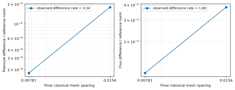
The finest classical field is a numerical reference, not an exact solution. First compare 32→64 and 64→128 in physical norms. The plotted difference rate is a reference-resolution indicator; two consecutive differences do not constitute a rigorous reference-error bound.
references = []
reference_dimensions = []
for resolution in (32, 64, 128):
    fine_global = TriangleMesh.unit_square(resolution)
    A_ref, _, F_ref = user_volume_forms(fine_global, 2)
    _, xy = nodal_space(fine_global, 2)
    boundary = np.flatnonzero(np.any(np.isclose(xy, 0) | np.isclose(xy, 1), axis=1))
    p_ref = dirichlet_solve(A_ref, F_ref, boundary, np.zeros(len(boundary)))
    references.append(ScalarField(fine_global, 2, p_ref))
    reference_dimensions.append(
        {
            "squares_per_direction": resolution,
            "triangles": len(fine_global.cells),
            "free_unknowns": len(p_ref) - len(boundary),
        }
    )
    print(reference_dimensions[-1])
reference = references[-1]
reference_refinement = [
    compare_scalar_fields((coarser,), finer, permeability, order=8)
    for coarser, finer in zip(references[:-1], references[1:])
]
for interval, norms in zip(("32 → 64", "64 → 128"), reference_refinement):
    print(interval, norms)

# These rates concern differences between successive reference meshes.
# They are indicators, not exact-solution error rates.
refinement_figure = plot_reference_differences(
    [1 / 64, 1 / 128],
    reference_refinement,
)

plt.show()

# A reference must resolve its own physical fields before serving as a baseline.
assert reference_refinement[-1]["pressure_relative"] < reference_refinement[0]["pressure_relative"]
assert reference_refinement[-1]["flux_relative"] < reference_refinement[0]["flux_relative"]
32 → 64 {'pressure_L2': 3.823696684608936e-05, 'flux_L2': 0.0073346478106178165, 'flux_energy': 0.005272480435871399, 'pressure_relative': 0.0018001151790877515, 'flux_relative': 0.03838323140026158, 'energy_relative': 0.03921980440020735}
64 → 128 {'pressure_L2': 3.7669518113256023e-06, 'flux_L2': 0.0021132796164602475, 'flux_energy': 0.0015405697662049793, 'pressure_relative': 0.00017731712073356501, 'flux_relative': 0.011059633117206041, 'energy_relative': 0.011458909837941546}
7. Compare pressure and physical flux on a common fine partition
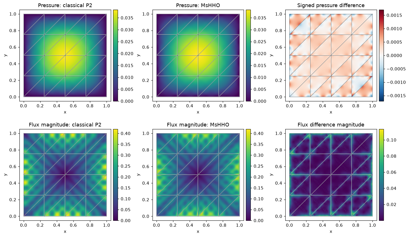
The reference mesh resolves every local mesh interface in this nested, uniformly refined case. Integrate on its triangles and use its field norms as denominators:
The comparison code keeps the coefficient inside flux and energy norms. Quadrature orders 8 and 10 independently check norm integration. At volume quadrature points, evaluate the original coefficients directly; do not compare images or interpolated color maps.
For plotting, sample every fine triangle separately. Duplicate interface points retain separate incident values. Pressure and flux-magnitude panels share scales with their reference panels; each difference has its own colorbar. All panels show the actual macro mesh.
errors_q8 = compare_scalar_fields(physical_fields, reference, permeability, order=8)
errors_q10 = compare_scalar_fields(physical_fields, reference, permeability, order=10)
quadrature_difference = max(
    abs(errors_q8[key] - errors_q10[key]) / max(abs(errors_q10[key]), np.finfo(float).tiny)
    for key in ("pressure_L2", "flux_L2", "flux_energy")
)
print(
    {"physical_relative_errors": errors_q10, "relative_norm_change_q8_q10": quadrature_difference}
)
assert quadrature_difference < 1e-5

figure = plot_scalar_comparison(
    macro,
    physical_fields,
    reference,
    permeability,
    numerical_label="MsHHO",
)
plt.show()
{'physical_relative_errors': {'pressure_L2': 0.000349696801857094, 'flux_L2': 0.022527859850014417, 'flux_energy': 0.01575881879143392, 'pressure_relative': 0.016460850348179897, 'flux_relative': 0.1178972545404677, 'energy_relative': 0.11721564816135271}, 'relative_norm_change_q8_q10': 1.860243788438027e-15}
Optional: use a prepared operator for this weak form
For the scalar diffusion form written above, scalar_operators provides a
portable Basix assembly convenience. Defining a new physical operator does not
require this function: the main computation already assembles the UFL expression
written by the user. The following check verifies agreement in the same local
finite-element space and basis before substituting this convenience.
from pymhm.fem.scalar.triangle import scalar_operators

A_prepared, M_prepared, F_prepared = scalar_operators(
    first_fine,
    local_degree,
    diffusion=permeability,
    source=source,
    order=assembly_order,
)
form_equivalence = {
    "stiffness_relative": float(
        sparse.linalg.norm(A_ufl - A_prepared) / sparse.linalg.norm(A_prepared)
    ),
    "mass_relative": float(sparse.linalg.norm(M_ufl - M_prepared) / sparse.linalg.norm(M_prepared)),
    "source_relative": float(np.linalg.norm(F_ufl - F_prepared) / np.linalg.norm(F_prepared)),
}
assert max(form_equivalence.values()) < 1e-10
print(form_equivalence)
{'stiffness_relative': 1.6755633221035159e-15, 'mass_relative': 1.410965141920348e-15, 'source_relative': 1.0931848206312767e-15}
record = {
    "method": "MsHHO",
    "physical_problem": f"-div(aε grad(p))={source:g}, p|boundary=0",
    "source": float(source),
    "epsilon": epsilon,
    "macro_triangles": len(macro.cells),
    "local_refinement": local_refinement,
    "local_degree": local_degree,
    "assembly_order": assembly_order,
    "error_orders": [8, 10],
    "global_free_unknowns": global_free_unknowns,
    "reference_dimensions": reference_dimensions,
    "reference_refinement": reference_refinement,
    "physical_errors": errors_q10,
    "quadrature_relative_difference": quadrature_difference,
    "global_residual": solution.residual,
    "diagnostics": diagnostics,
    "basis_digests": basis_digests,
    "form_equivalence": form_equivalence,
}
print(
    save_scalar_report(
        ROOT,
        "mshho_multiscale",
        record,
        archive,
        {
            "physical-fields": figure,
            "permeability": fig_material,
            "reference-refinement": refinement_figure,
        },
    )
)
./build/docs-restructure/final-workspaces/provenance-final-mshho_multiscale-ef542e24d568/build/introduction/mshho_multiscale
8. Separate smooth source and energy convergence
The oscillatory material study above is distinct from this smooth convergence control. Use identity diffusion on the unit square and independently differentiated data
Exterior pressure is zero. Keep matching P0 cell and face moments (\(m=\ell=0\)), the projected-source variant and local P3 energy reconstruction with two edge subdivisions. Refine \(n=1,2,4,8,16,32\) while preserving these spaces.
Theorem 6.3 of Chaumont-Frelet, Ern, Lemaire and Valentin (2022) assumes \(f\in H^{m+1}(\mathcal T_H)\) and \(K\nabla p\in H^{\ell+1}(\mathcal T_H)\) on regular matching macrocell submeshes. For exact local PDE reconstructions, it separates the source and flux terms:
The ideal estimate gives first-order energy here. With \(K=I\), physical-flux error equals broken-gradient error. Second-order pressure is an observation, rather than a conclusion of this energy theorem. The executed P3/r2 Galerkin realization remains a finite local solve; the local-resolution control below measures its contribution for these homogeneous data. Its smooth rates do not transfer to heterogeneous coefficients, unresolved local responses or singular domains.
Recompute every measured order
For successive physical errors \(E_{i-1},E_i\) at the actual macro diameters, compute
The cell reads the attributed numerical record, displays every measured level and recomputes its orders. It does not execute a PDE acquisition. The fitted terminal slope uses the final four levels and their three intervals. For each declared target \(q\), the amplitude ratio is the maximum divided by the minimum of \(E/H^q\) over those same levels. A value near one indicates stabilization of the compensated error; an observed L2 order is kept separate from a proved energy estimate.
import json
from IPython.display import Markdown, display
from examples.tutorial_convergence import refinement_series, asymptotic_summary, plot_method_series
refinement_record = ROOT / 'examples/results/tutorial-methods/mshho-current.json'
refinement_data = json.loads(refinement_record.read_text(encoding='utf-8'))
refinement_rows = refinement_data['rows']
refinement_error_keys = {'pressure L2': 'pressure_l2', 'physical Darcy flux L2': 'flux_l2'}
refinement_targets = {'physical Darcy flux L2': 1.0}
refinement_rows = sorted(refinement_rows, key=lambda refinement_row: refinement_row['macro_diameter'], reverse=True)
refinement_sizes = np.asarray([refinement_row['macro_diameter'] for refinement_row in refinement_rows])
refinement_field_errors = {refinement_field: np.asarray([refinement_row[refinement_key] for refinement_row in refinement_rows]) for refinement_field, refinement_key in refinement_error_keys.items()}
refinement_orders = {refinement_field: np.log(refinement_values[:-1] / refinement_values[1:]) / np.log(refinement_sizes[:-1] / refinement_sizes[1:]) for refinement_field, refinement_values in refinement_field_errors.items()}
refinement_header = ['Refinement size'] + [refinement_column for refinement_field in refinement_error_keys for refinement_column in (refinement_field, 'Order')]
refinement_lines = [' | '.join(refinement_header), ' | '.join(['---'] * len(refinement_header))]
for refinement_index, refinement_size in enumerate(refinement_sizes):
    refinement_values = [f'{refinement_size:.6g}']
    for refinement_field in refinement_error_keys:
        refinement_values.extend([f'{refinement_field_errors[refinement_field][refinement_index]:.6e}', '—' if refinement_index == 0 else f'{refinement_orders[refinement_field][refinement_index - 1]:.3f}'])
    refinement_lines.append(' | '.join(refinement_values))
display(Markdown('\n'.join(refinement_lines)))
refinement_series_data = refinement_series(refinement_record, refinement_rows, 'macro_diameter', refinement_error_keys, refinement_targets, method='mshho', spaces='P0 cell and face moments; P3/r2 energy reconstruction; projected source', rate_provenance='Chaumont-Frelet et al. (2022), Theorem 6.3: first-order energy for exact local PDE reconstructions, source in H^1 and A grad(p) in H^1 on regular matching macrocell submeshes; finite P3/r2 reconstruction adds local approximation error; pressure order two observed separately.', root=ROOT)
print({'record': refinement_series_data['record'], 'sha256': refinement_series_data['sha256']})
for refinement_field, refinement_summary in asymptotic_summary(refinement_series_data).items():
    print(refinement_field, {'last_three_orders': [round(refinement_order, 3) for refinement_order in refinement_summary['orders']], 'fitted_order': round(refinement_summary['fitted_order'], 3), 'target': refinement_summary['target'], 'normalized_amplitude_ratio': refinement_summary.get('amplitude_ratio')})
plot_method_series(refinement_series_data)
plt.show()
| Refinement size | pressure L2 | Order | physical Darcy flux L2 | Order |
|---|---|---|---|---|
| 1.41421 | 1.368302e-01 | — | 1.056841e+00 | — |
| 0.707107 | 1.001886e-01 | 0.450 | 9.830652e-01 | 0.104 |
| 0.353553 | 2.681001e-02 | 1.902 | 5.019038e-01 | 0.970 |
| 0.176777 | 6.791185e-03 | 1.981 | 2.516432e-01 | 0.996 |
| 0.0883883 | 1.703111e-03 | 1.995 | 1.258917e-01 | 0.999 |
| 0.0441942 | 4.261102e-04 | 1.999 | 6.295424e-02 | 1.000 |
{'record': 'examples/results/tutorial-methods/mshho-current.json', 'sha256': 'bfdd177ea0910690cb9a909a49bf404936858d3a988078d231d4571956ce5c44'}
pressure L2 {'last_three_orders': [1.981, 1.995, 1.999], 'fitted_order': 1.992, 'target': None, 'normalized_amplitude_ratio': None}
physical Darcy flux L2 {'last_three_orders': [0.996, 0.999, 1.0], 'fitted_order': 0.998, 'target': 1.0, 'normalized_amplitude_ratio': 1.0034471025178162}
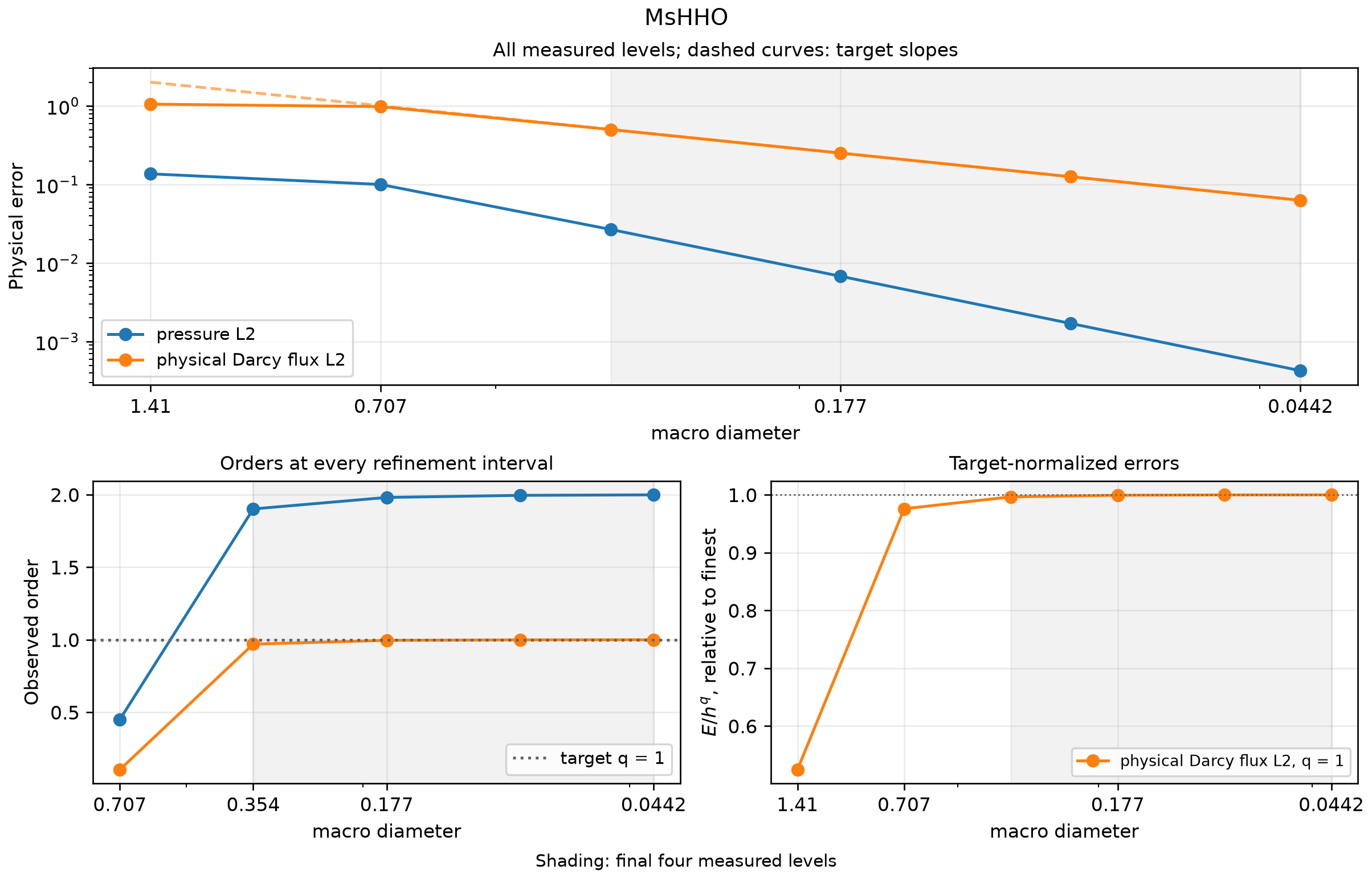
Download the figure as SVG or PDF. Shading covers the same final four levels in every panel; dashed curves are target powers anchored to the finest measured error.
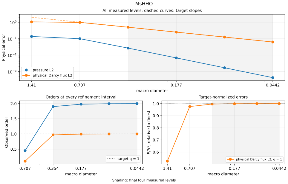
The current acquisition compares full physical norms at error quadrature orders 10 and 12; the largest relative difference over all levels and fields is 1.577e-14. It also checks the original method equations in their declared coefficient coordinates, retaining global compatibility, local reconstruction and physical field errors as separate quantities. Its source closure is unchanged during execution. The norm-only record contains no persisted coefficient vector.
Local Galerkin sensitivity at fixed macro resolution
Hold \(n=8\), the physical data and all trace spaces fixed, and double only the local subdivisions from 2 to 4. Pairwise differences are integrated on the nested finer partition using the executed coefficient bases. Discontinuous pressure and independent interface values remain separate. Both solutions are also compared directly with the analytical fields:
| Field | Coarse error | Refined error | Field difference | Difference / coarse error |
|---|---|---|---|---|
| pressure L2 | 6.791185e-03 | 6.791185e-03 | 1.124624e-14 | 1.656e-12 |
| physical Darcy flux L2 | 2.516432e-01 | 2.516432e-01 | 5.324106e-14 | 2.116e-13 |
For this constant coefficient and projected P0 source, the local reconstructions can be represented in the P3 spaces. The r2/r4 physical fields agree at roundoff in this measurement. This statement applies to this homogeneous qualification; heterogeneous coefficients require their own local-resolution control.
The full physical-error norms agree at quadrature orders 10 and 12, with maximum relative change 1.332e-15. For the two-grid sensitivity, the change in the integrated field difference divided by the coarse analytical error is 3.200e-15. This scale assesses the local contribution to that physical error and remains meaningful when the two fields differ only at roundoff. The raw differences at both quadrature orders and their unscaled relative changes remain in the local-control record (SHA256 8933c2e8c4f68a626276c4a0fc8e1b06e14334f8f8c413a2649137de27fe2350). Original equations and reconstruction constraints retain their separate unchanged checks.
The smooth convergence figure uses the attributed numerical record (SHA256 bfdd177ea0910690cb9a909a49bf404936858d3a988078d231d4571956ce5c44). The shared rate notebook compares the method sequences.
Reproduce this tutorial
View the source notebook or download the notebook, then open it:
The first cell downloads a SHA256-verified companion containing inspectable support files. Downloading does not execute them. Native UFL forms require the compatible backend described in the installation guide.
For batch execution, extract the same companion, change to its workspace and run:
The runner uses the active interpreter and writes an executed copy and receipt under build/notebooks/introduction/. Larger field archives have documented downloads.
Figures and outputs of sections 1–7 retain notebook SHA256 bf74f41c2a8e6dfa7e0cd323dec66d951c5e43f086adbcacb595ca751253dd10 in the publication manifest. The smooth convergence figure and tables use the separate numerical records cited in section 8. Running the current source produces a receipt for its actual notebook, support files and environment.
References
- Théophile Chaumont-Frelet, Alexandre Ern, Simon Lemaire, and Frédéric Valentin (2022). Bridging the Multiscale Hybrid-Mixed and Multiscale Hybrid High-Order Methods, ESAIM: M2AN 56, 261–285. DOI: 10.1051/m2an/2021082.