Conservative RAD on star-shaped polyhedra

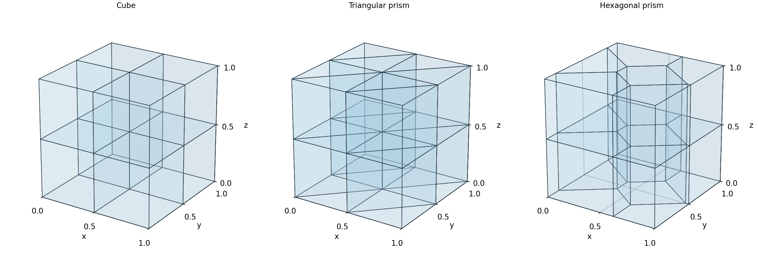
PolyhedralMesh keeps each planar polygonal macroface as a single entity. Continuous tetrahedral local spaces solve the interior problems, while PolygonalSkeleton3D supplies one constant or one affine polynomial on each original macroface. Triangulation diagonals carry no independent global traces. This realizes the polyhedral geometry allowed by the generalized RAD formulation of Araya et al. (2024).

Geometry and spaces

The native geometry accepts conforming star-shaped cells with planar simple polygonal faces, including nonconvex cells and concave faces. Face vertices are cyclically ordered. Each cell has a closed, connected, orientable boundary; shared faces have opposing outward orientations. An interior kernel point and its positive distance from every face plane certify a kernel ball. Its radius is recorded in kernel_radii. The star-shaped-ball hypothesis is the geometric condition in §4.1(iii) of the cited RAD analysis. Uniform family regularity additionally needs a lower bound on kernel radius divided by cell diameter.

Convex faces retain their deterministic fan triangulation. Concave faces use a conforming ear triangulation. Cones from the certified cell center to these triangles form the local tetrahedral mesh; a separating-axis check rejects positive-volume overlaps between cones. The construction preserves reentrant notches and never fills a convex hull. Curved faces, separate cavity shells and empty kernels are rejected. Coplanar adjacent polygons may remain distinct macrofaces, with separate physical moments.

Optional dyadic refinement identifies shared nodes by integer barycentric topology. Local fields are continuous Pk across these tetrahedra; the basis accepts arbitrary positive degree and the chosen formulation still requires adequate quadrature and compatible trace coupling. The additional nonconvex campaign verifies five L-prism/cuboid resolutions and a native UFL full-saddle comparison on two reentrant cells.

A \(P_0\) macroface has one degree of freedom. A \(P_1\) macroface has three, regardless of its vertex count or triangulation:

\[ \lambda_F(x)=a_F+b_F\frac{(x-c_F)\cdot t_{F,1}}{\sqrt{|F|}} +c_F^{\lambda}\frac{(x-c_F)\cdot t_{F,2}}{\sqrt{|F|}}. \]

Here \(c_F\) is the area centroid and the tangents are orthonormal. Coefficients refer to the canonical normal directed outward from the first neighboring cell. Local coupling includes the corresponding orientation sign. External Robin values are projected onto this same polynomial space by a physical \(L^2(F)\) projection.

The local and skeletal spaces must have sufficient independent coupling. The solver checks the condensed system's numerical rank. In particular, an unrefined cubic macrocell with local \(P_2\) and face \(P_1\) contains an invisible trace mode; it is rejected. The \(P_4/P_1\) campaign below and the reported \(P_3/P_1\) affine patches satisfy the checked discrete coupling. The 2024 analysis gives the sufficient 3D degree condition \(k\ge\ell+3\) under its facet-matching Assumptions A1–A2. Thus P4/P1 meets that degree condition; the P3/P1 patches establish finite polynomial reproduction and rank, without claiming the theorem's general error estimate.

PDE and boundary convention

The conservative equation is

\[ -\nabla\cdot(K\nabla u)+\nabla\cdot(\beta u)+cu=f. \]

The local form uses skew transport and the effective reaction \(c+\nabla\cdot\beta/2\). Its natural multiplier is \(\lambda=(-K\nabla u+\beta u/2)\cdot n\), whereas the physical flux evaluated by the solution is \(-K\nabla u+\beta u\). Dirichlet data enter the global weak moments on the remaining exterior faces. Variable velocity requires an explicit divergence; SUPG with variable diffusion also requires \(\nabla\cdot K\).

Physical constant modes are retained by default, including near-singular local operators. The explicit coarse_space="kernel" policy retains only genuine constant null modes. An all-Robin problem admits a physical mean when reaction vanishes and the velocity is divergence-free and tangent to the full exterior. The original physical equations are checked after imposing this mean.

The example helpers below are repository sources, supplied separately from the installed library. Open the corresponding notebook to acquire its verified companion, as described in the notebook guide.

import numpy as np
from pymhm import assemble
from pymhm.meshes.polyhedral import PolyhedralMesh
from examples.formulations.transport_3d import define_transport_3d
from examples.formulations.scalar_3d import scalar_constraints_3d, recover_transport_3d

mesh = PolyhedralMesh.cubes(2)
definition = define_transport_3d(
    mesh,
    degree=4,
    diffusion=0.1,
    velocity=(1.0, 0.0, 0.0),
    source=lambda x: np.ones(len(x)),
)
system = assemble(definition.problem)
coefficients = system.solve(constraints=scalar_constraints_3d(definition, system))
solution = recover_transport_3d(definition, system, coefficients)

The user-defined provider in examples/formulations/scalar_3d.py composes the public tetra_transport_operators, polygonal_trace_coupling and boundary projection with explicit four-block equations. Natural data, coefficient derivatives, Galerkin/SUPG, retained constants or selective kernels, and a physical mean use the same declarations as the tetrahedral example. Assembly supports serial, thread and spawn workers through generic ExecutionConfig; SolverConfig declares independent local/global solvers and arithmetic for iterative refinement. Original polygonal faces retain their unknowns throughout.

Analytical campaign

On the unit cube, the smooth three-dimensional data from §5.2.1 are

\[ \begin{aligned} K&=0.1I,\qquad \beta=(1,0,0),\qquad c=0,\\ u&=\sin(6\pi x)\sin(4\pi y)\sin(2\pi z),\\ f&=5.6\pi^2u+\partial_xu. \end{aligned} \]

All exterior Dirichlet values vanish. The campaign uses local \(P_4\) and one \(P_1\) polynomial per original face, with five independently specified macro resolutions. The three families are cubes, triangular prisms and extruded convex Voronoi polygons; the latter include nonquadrilateral polygonal faces. These are original meshes with the published PDE and degrees, not the article's unavailable historical mesh realization.

Assembly uses eight Duffy points per coordinate. Positive error quadrature uses ten, with a twelve-point scalar-error check on each family's finest mesh. The energy-space norm is \(\|e\|_V=(\|\nabla e\|^2+\|e\|^2/3)^{1/2}\), since the squared diameter of the unit cube is three. The physical flux error includes advection.

Macro family	\(n\)	Cells	\(L^2\) error	\(V\) error	Physical flux \(L^2\) error
cube	2	8	0.158999	5.329271	0.563130
cube	3	27	0.171405	4.444685	0.480116
cube	4	64	0.098837	3.321122	0.345042
cube	5	125	0.054512	2.134023	0.221299
cube	6	216	0.040224	1.906931	0.194558
triangular prism	2	16	0.313256	6.812927	0.741945
triangular prism	3	54	0.212936	5.342275	0.572471
triangular prism	4	128	0.130207	4.030258	0.413215
triangular prism	5	250	0.063167	2.428163	0.247054
triangular prism	6	432	0.047967	2.169592	0.219416
hexagonal prism	2	12	0.185123	4.769644	0.530109
hexagonal prism	3	36	0.148823	3.774670	0.406549
hexagonal prism	4	80	0.066044	2.264220	0.239593
hexagonal prism	5	150	0.040584	1.668919	0.172123
hexagonal prism	6	252	0.025304	1.230969	0.124348

The largest relative change of the finest scalar error under the ten-to-twelve point quadrature check is \(1.28\times10^{-11}\). All fifteen original-system backward residuals are below \(1.16\times10^{-15}\). These checks address integration and algebra; the measured analytical errors quantify discretization.

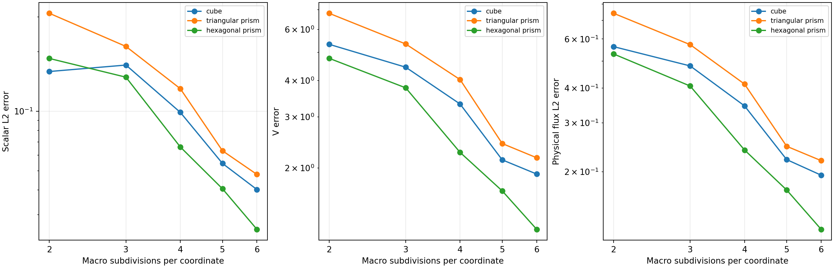
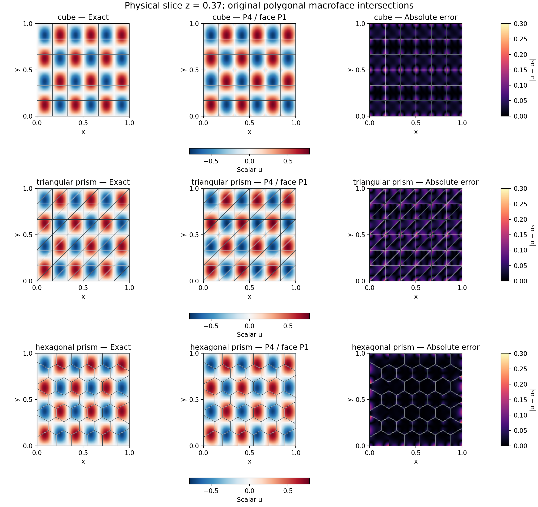
Slice samples at \(z=0.37\) are evaluated in their owning tetrahedron; values on distinct macrocells are not averaged. Macro outlines are the intersections of the actual polyhedral faces with the slice. The maps illustrate fields; norms use volume integration. Coarse grids can display nonmonotonic scalar errors for this oscillatory solution, so the records retain every measured level. The field replay record identifies the finest-resolution coefficients and their agreement with the original physical error measurements for all three macroelement families.

Verification and reproduction

Tests verify exact volume and surface area, the divergence theorem for affine fields, two cells sharing a quadrilateral face, and invariance under cyclic face reversal and face-list reordering. They also cover full physical RAD patches, variable-coefficient SUPG, Neumann projection, mean gauges, selective constant modes, incompatible data and serial/process equivalence. The local finite-element operators are shared with the independently checked tetrahedral RAD implementation. Eight native Basix/UFL checks independently integrate \(P_3/P_4\) test functions against affine polygonal-face loads on cubes, shared faces, hexagonal prisms and distinct coplanar faces.

pixi run --locked -e notebooks python -m examples.solve_polyhedral_rad --workers 4
pixi run --locked -e notebooks python -m examples.plot_polyhedral_rad

Numerical summaries and source hashes are in examples/results/polyhedral-rad.json; local coefficients used by the figures are in build/results/polyhedral-rad. Notebook 49 reads those summaries and figures without rerunning the campaign.

References

• Rodolfo Araya, Fabrice Jaillet, Diego Paredes, and Frédéric Valentin (2024). Generalizing the multiscale hybrid-mixed method for reactive-advective-diffusive equations, Computer Methods in Applied Mechanics and Engineering 428, 117089. DOI: 10.1016/j.cma.2024.117089.