Flux and conforming potential recovery
Executable notebook · Download notebook
This tutorial first declares the local and global equations, then reconstructs physical fields from their solution. The refined analytical study uses the data of Barrenechea et al. (2026), §6.1: \(p=\sin(2\pi x)\sin(2\pi y)\), \(K=I\), \(f=8\pi^2p\), and homogeneous Dirichlet pressure on the unit square. The approximation spaces and mesh ratios are stated explicitly; the numerical observations are PyMHM computations with these data, rather than an assertion of identical published table ordinates.
The workflow is meshes → local equations → global balance → assemble → solve → recovered fields → independently integrated errors. Install the native UFL backend following the installation guide.
1. Declare analytical fields and the source
The NumPy gradient and source are differentiated independently from the UFL volume form. The exact physical Darcy flux is \(q=-\nabla p\).
import numpy as np
import matplotlib.pyplot as plt
import ufl
from pymhm import (
    Equation, FaceSpace, LocalContext, MeshHierarchy, SkeletonSpace, TriangleMesh,
    assemble, bind_interface, bind_problem, columns, solve,
)
from pymhm.postprocessing.solutions import DarcySolution
from pymhm.recovery.moments import reconstruct_darcy_moments
from pymhm.estimators.darcy import estimate_darcy_error
from pymhm.adaptivity.darcy import mark_dorfler
from threadpoolctl import threadpool_limits


def exact_pressure(points: np.ndarray) -> np.ndarray:
    """Analytical pressure; it vanishes on every exterior edge."""
    return np.sin(2 * np.pi * points[:, 0]) * np.sin(2 * np.pi * points[:, 1])


def exact_gradient(points: np.ndarray) -> np.ndarray:
    """Independently differentiated physical pressure gradient."""
    x, y = 2 * np.pi * points.T
    return 2 * np.pi * np.column_stack((np.cos(x) * np.sin(y), np.sin(x) * np.cos(y)))


def source(points: np.ndarray) -> np.ndarray:
    """Negative Laplacian computed independently of the discrete operator."""
    return 8 * np.pi**2 * exact_pressure(points)
2. Choose compatible spaces and bind their interface
The field illustration uses 512 macrotriangles, each containing four fine triangles. The convergence study uses \(n=4,8,16,32\) subdivisions per coordinate, \(H=\sqrt{2}/n\), and \(h=H/2\). Trace degree \(\ell=0\) uses P2 local pressure; \(\ell=1\) uses P3. RT reconstruction degree \(m=2\) satisfies \(k\ge\ell+2\) and \(\ell\le m\le k\) in both branches. Convex macrocells and a conforming fine triangulation satisfy the estimator's geometric hypotheses.
macro = TriangleMesh.unit_square(16)
local_meshes = tuple(macro.submesh(cell, 2) for cell in range(len(macro.cells)))
hierarchy = MeshHierarchy(macro, local_meshes)
skeleton = SkeletonSpace(macro, tuple(FaceSpace.uniform(1) for _ in macro.faces))
interface = bind_interface(skeleton, convention="normal")
3. Write the variational formulation as UFL
The local physical volume moment fixes the constant complement and retains one mean per macrocell. The minus sign in the global pairing is mathematical; the interface binding supplies numbering and normal orientation.
def local_equations(local: LocalContext, degree: int = 3, forcing=None):
    """Declare primal diffusion, independent trace tests and physical mean."""
    space = local.native_space(degree=degree)
    p, v = ufl.TrialFunction(space.space), ufl.TestFunction(space.space)
    x = ufl.SpatialCoordinate(space.mesh)
    dx = ufl.Measure("dx", domain=space.mesh, metadata={"quadrature_degree": 20})
    forcing = (8 * np.pi**2 * ufl.sin(2 * np.pi * x[0]) * ufl.sin(2 * np.pi * x[1])
               if forcing is None else forcing(space.mesh))
    local.field("pressure", space)
    return local.equations(
        a=ufl.inner(ufl.grad(p), ufl.grad(v)) * dx,
        L=forcing * v * dx,
        b=local.trace_pairings(lambda phi, ds: phi * v * ds),
        c=local.trace_pairings(lambda phi, ds: -phi * p * ds, axis="rows"),
        kernel=np.ones((space.size, 1)), moments=columns(v * dx),
    )
def global_equation(global_context):
    """Supply the weak Dirichlet moments in the bound interface layout."""
    boundary, fixed = global_context.boundary_data(0.0, order=8)
    assert not fixed
    return Equation(0, global_context.trace_load(-boundary))


problem = bind_problem(hierarchy, interface, local_equations,
                       global_equation=global_equation, retained=1)
4. Assemble, solve and retain the executed field basis
with threadpool_limits(1):
    system = assemble(problem)
    coefficients = solve(system)
pressure_fields = coefficients.field("pressure")
solution = DarcySolution(
    skeleton=skeleton, local_meshes=local_meshes,
    pressure=tuple(field.portable_coefficients for field in pressure_fields),
    flux=tuple(-field.gradient(mesh.points[mesh.cells].mean(axis=1),
                               cells=np.arange(len(mesh.cells)))
               for mesh, field in zip(local_meshes, pressure_fields, strict=True)),
    hybrid=coefficients, formulation="primal", permeability=1.0,
    source=source, degree=3, quadrature_order=16,
)
print({"global_original_compatibility": coefficients.raw_residual,
       "pressure_L2": solution.l2_error(exact_pressure, order=12)})
DarcySolution is a physical coefficient record; constructing it performs no
additional PDE solve. Native fields carry their executed basis and expose
portable_coefficients through that mapping.
coefficients.raw_residual measures the original global compatibility defect
of the assembled trace/retained system. It is not the norm of all local
volume equations, nor a physical field error. A separate native observer checks
every original local volume row and the original trace equations of the same
eight-subdivision solve, reusing the shared original-row diagnostic:
| Native eight-subdivision control | Maximum relative local volume rows | Full uncondensed rows / physical load |
|---|---|---|
| Sinusoidal P2/P0 | 3.321e-15 | 5.667e-15 |
| Sinusoidal P3/P1 | 1.040e-14 | 1.762e-14 |
| Localized P3/P1 | 4.196e-15 | 6.124e-15 |
| RT0-compatible sinusoidal P3/P0 | 1.376e-14 | 1.918e-14 |
These are Euclidean coefficient-row diagnostics with stated action/physical-load scales. They retain the unchanged \(10^{-10}\) gate and are distinct from physical volume norms and the reconstruction's normal/continuous-test invariants.
5. Recover the canonical H(div) flux
The canonical RT moments preserve the skeletal boundary normal moments, average the interior normal moments, and retain interior vector moments of the raw physical flux:
recovered = reconstruct_darcy_moments(solution, degree=2, quadrature_order=16)
normal_defect = max(np.max(abs(row)) for row in recovered.normal_flux_residuals())
continuous_defect = max(np.max(abs(row)) for row in recovered.continuous_moment_residuals())
assert normal_defect < 1e-10
assert continuous_defect < 1e-10
flux_error = recovered.flux_l2_error(lambda x: -exact_gradient(x), order=16)
projection_error = recovered.projected_divergence_l2_error(source, order=16)
The conservation identity is tested against continuous macro-local P2 functions. It does not impose every discontinuous fine-cell constant balance. The raw broken gradient, canonical RT flux, and independently equilibrated RT0 flux are three distinct fields.
6. Verify the asymptotic estimates on four refined levels
Theorem 4.7 and Remark 5.1 of the accepted author manuscript give, for the stated regularity and degree assumptions,
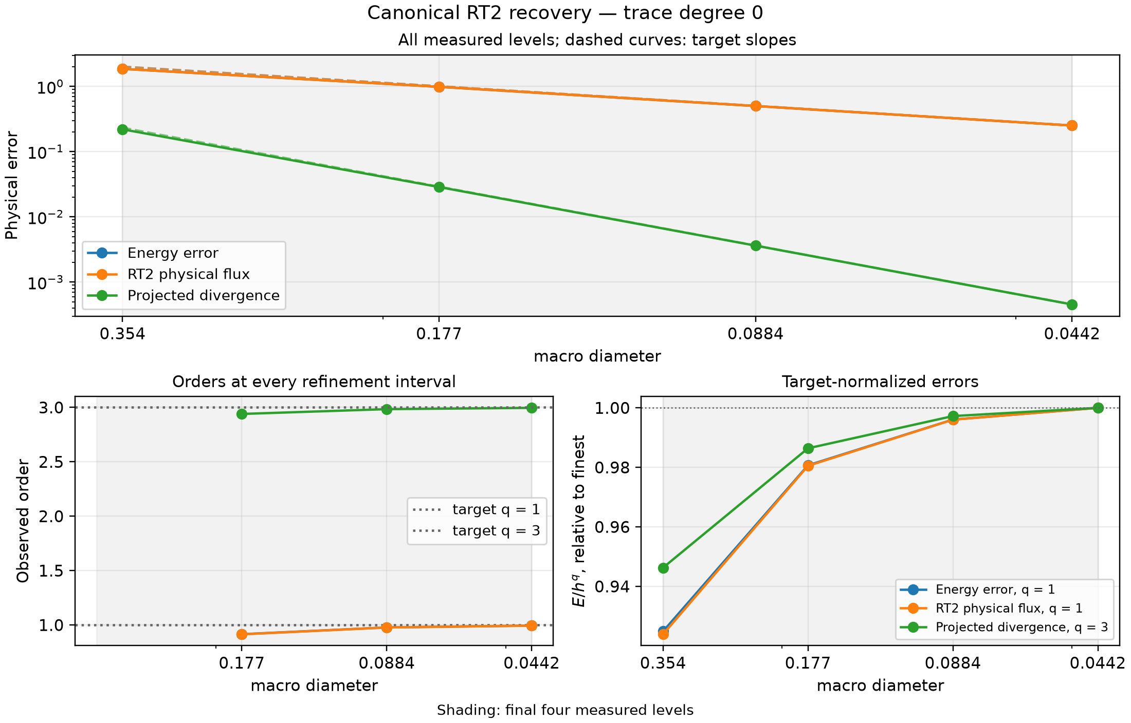
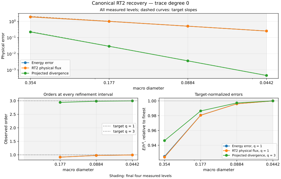
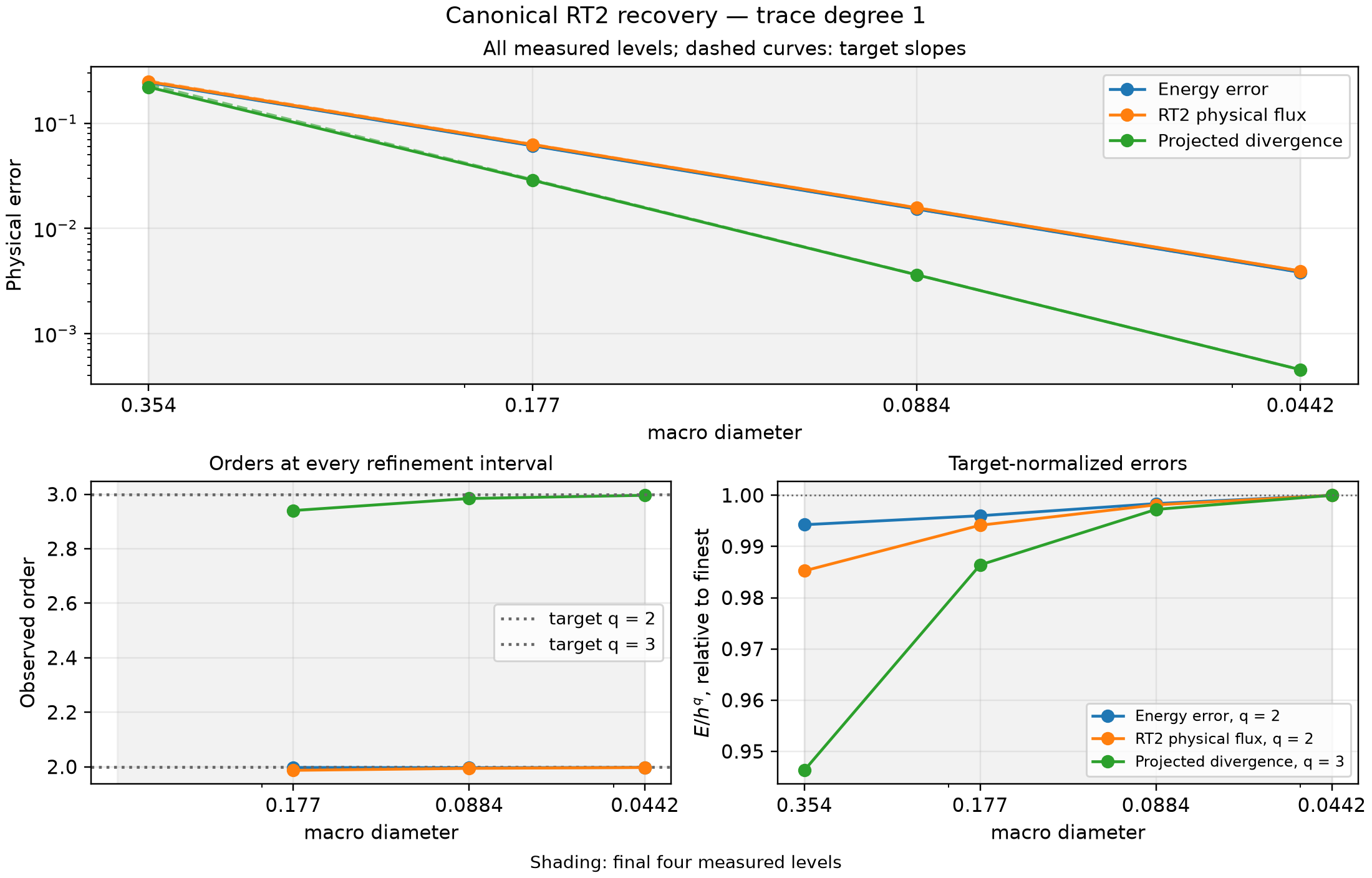
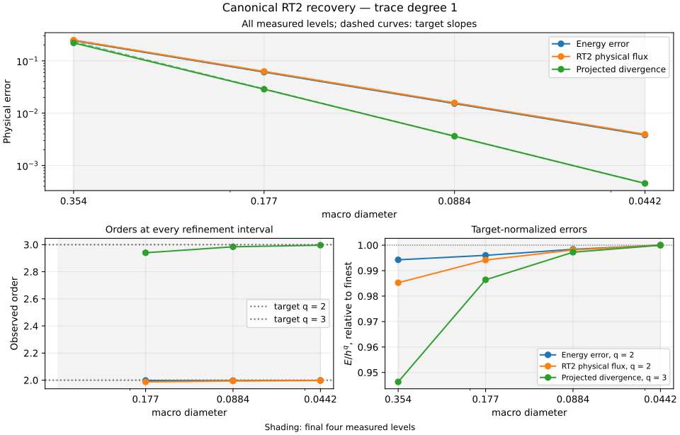
The flux estimate assumes diffusion polynomial on every fine triangle, \(p\in H^{k+1}(K)\) and \(A\nabla p\in H^{\ell+1}(K)^2\cap H(\mathrm{div};K)\), with Assumption A's compatible shape-regular partitions. Identity diffusion and the sine solution satisfy these conditions. The physical flux therefore has order one or two as \(\ell=0\) or \(1\). The projected divergence has order three. Here \(\Pi_{\Omega,2}\) acts separately on each macrotriangle: its range is continuous P2 on that macrotriangle's fine mesh, without continuity across macrofaces. The raw divergence is recorded separately and is not assigned the projected-divergence estimate. The projected bound additionally uses \(f\in H^3(K)\) and Assumption B's globally conforming fine mesh. In the displayed flux bound \(H\) is skeletal-subface diameter; macrocell diameter enters the estimator's Poincaré factor separately. Both norms are integrated with 12 and 16 Gauss points per Duffy coordinate; their difference is checked before accepting each level. The figures display every measured level, every successive order, and the normalized \(E/H^q\) plateau.
| Trace degree | Quantity | Three consecutive orders | Expected order | Max/min normalized amplitude |
|---|---|---|---|---|
| 0 | Energy error | 0.916, 0.978, 0.994 | 1 | 1.081 |
| 0 | RT2 physical flux | 0.914, 0.977, 0.994 | 1 | 1.082 |
| 0 | Projected divergence | 2.940, 2.984, 2.996 | 3 | 1.057 |
| 1 | Energy error | 1.997, 1.997, 1.998 | 2 | 1.006 |
| 1 | RT2 physical flux | 1.987, 1.994, 1.997 | 2 | 1.015 |
| 1 | Projected divergence | 2.940, 2.984, 2.996 | 3 | 1.057 |
The baseline is independently assembled classical conforming P3 Galerkin on \(16\times16\), \(32\times32\), and \(64\times64\) global square subdivisions. Its pressure and physical-flux errors against the analytical fields verify its own refinement. The analytical solution supplies the exact comparator.
| Global square subdivisions | P3 nodal unknowns | Pressure error | Physical vector-flux error |
|---|---|---|---|
| 16 × 16 | 2401 | 1.967367e-05 | 3.291818e-03 |
| 32 × 32 | 9409 | 1.204168e-06 | 4.107999e-04 |
| 64 × 64 | 37249 | 7.463012e-08 | 5.128221e-05 |
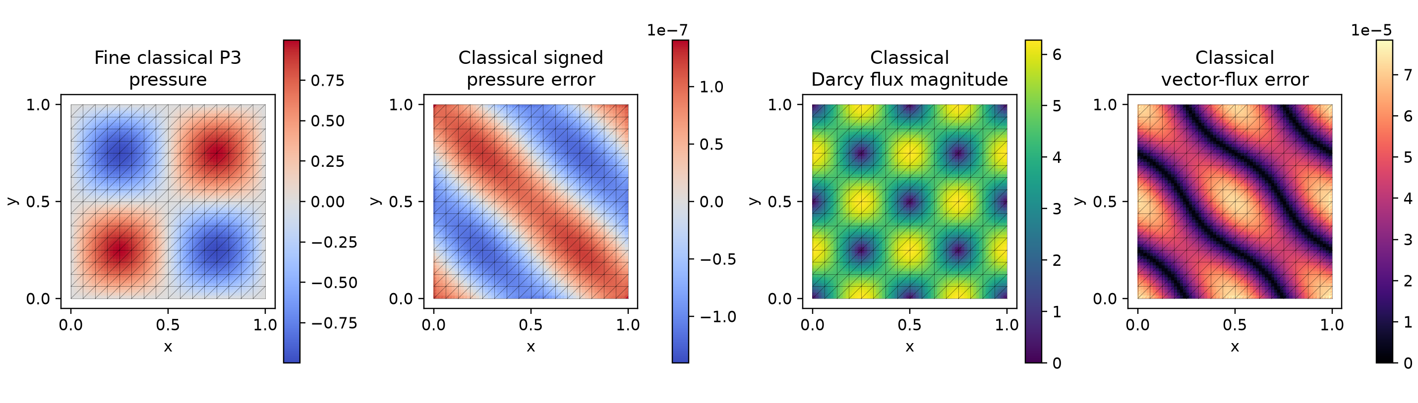
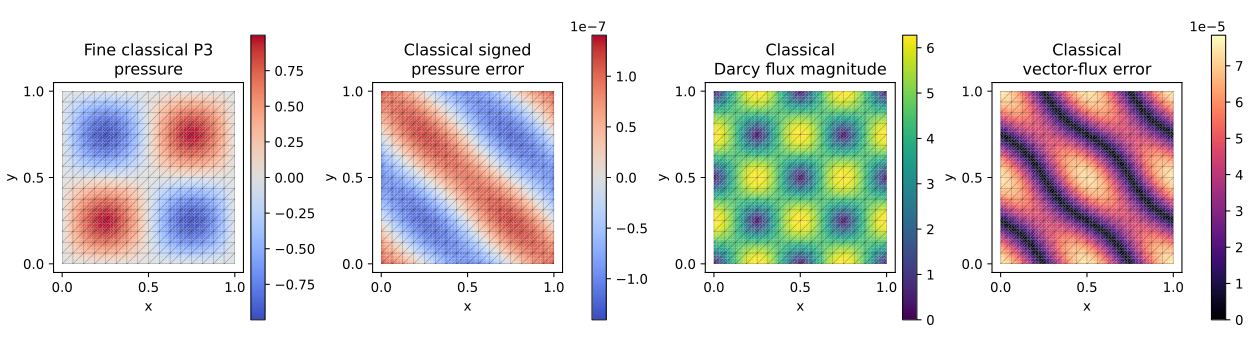
The global reference panels show the actual 64-subdivision solution with the 16-subdivision comparison macro mesh overlaid. These are distinct meshes. Pressure orders are 4.030 and 4.012; flux orders are 3.002 and 3.002.
7. Inspect fields on a resolved mesh
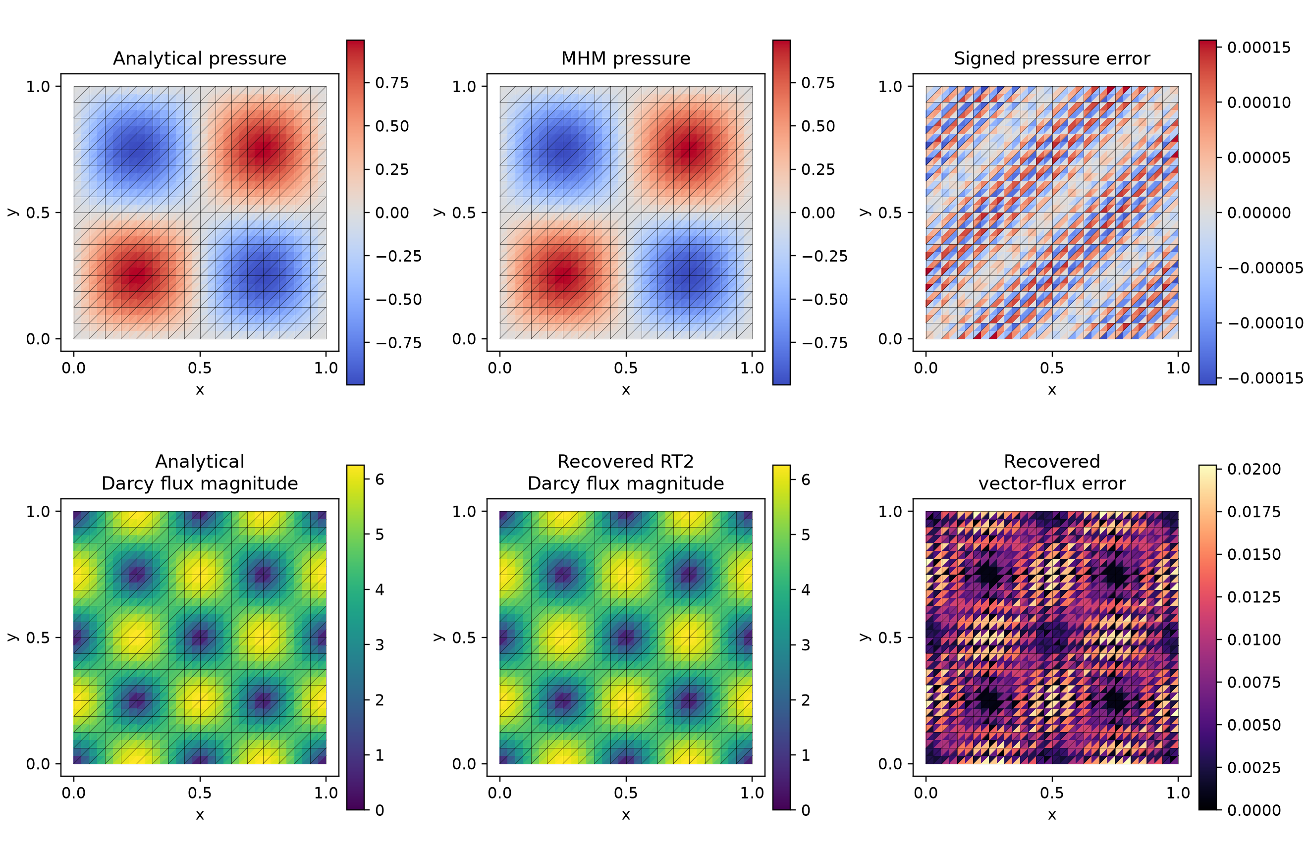
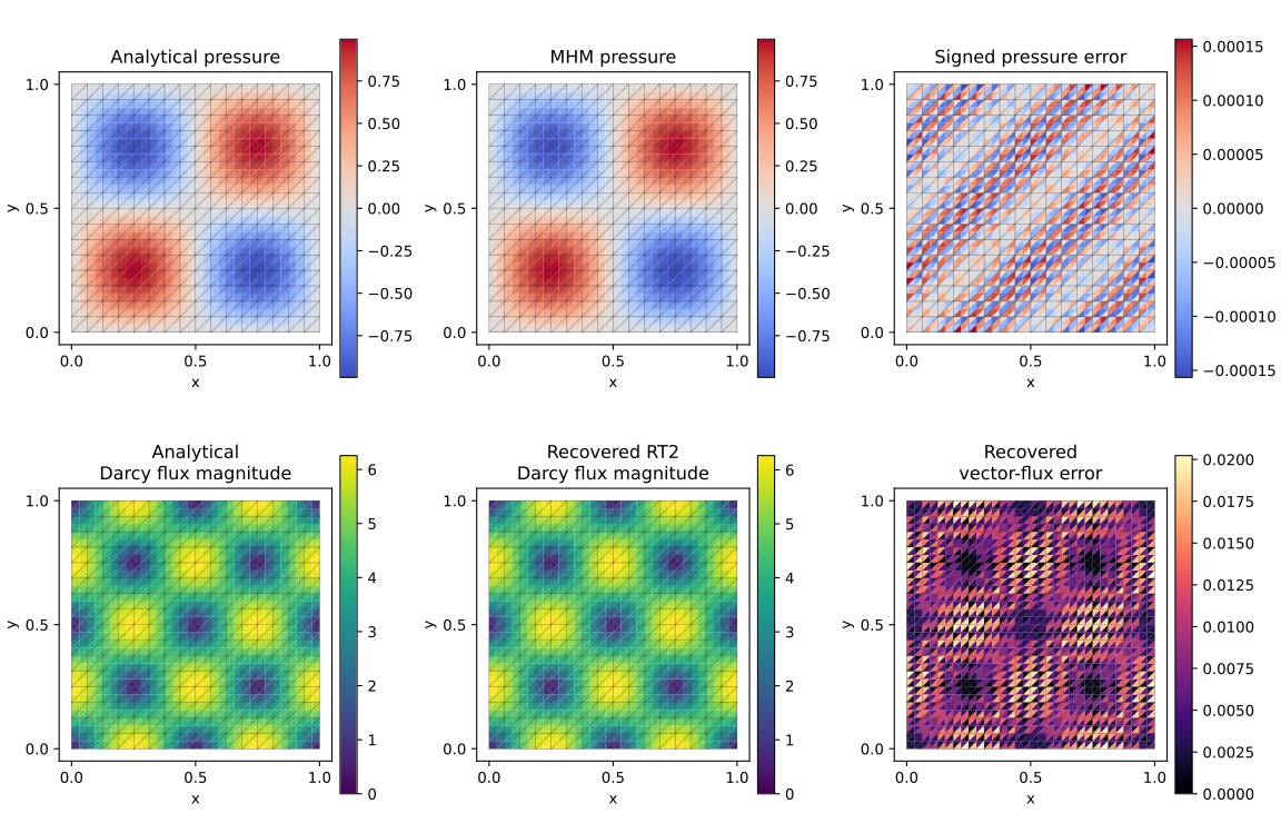
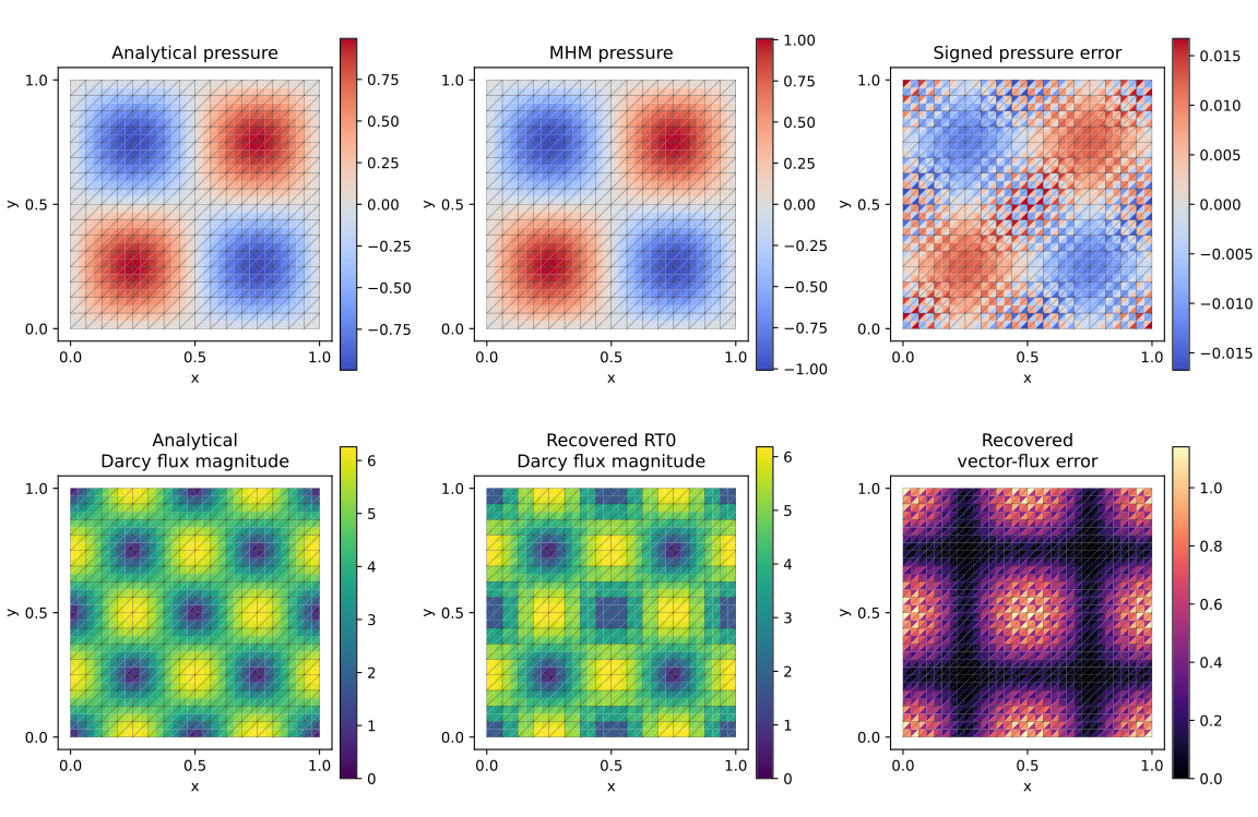
Every panel overlays the actual macro mesh and owns its color scale. Display samples are taken independently at each fine-triangle centroid; no averaging across an interface is used. Pressure error is signed; flux error is the magnitude of the vector difference. Error norms use volume quadrature.
8. Recover a conforming potential
from pymhm.estimators.darcy import recover_potential
potential = recover_potential(solution, homogeneous_dirichlet=True)
The Oswald potential averages incident finite-element nodal traces and imposes the declared homogeneous boundary values. It is a separate continuous Pk field. Its approximation error and boundary defect are reported in the notebook. The following integrated errors use the same independently checked rules and all four macro meshes; these potential orders are observations, rather than a new universal reconstruction estimate.
| Trace degree | Macro subdivisions | Conforming potential error | Consecutive observed order |
|---|---|---|---|
| 0 | 4 | 9.535888e-02 | — |
| 0 | 8 | 2.630156e-02 | 1.858 |
| 0 | 16 | 6.759941e-03 | 1.960 |
| 0 | 32 | 1.703478e-03 | 1.989 |
| 1 | 4 | 4.687328e-03 | — |
| 1 | 8 | 5.518882e-04 | 3.086 |
| 1 | 16 | 6.893670e-05 | 3.001 |
| 1 | 32 | 8.671578e-06 | 2.991 |
9. Equilibrate an RT0 flux with strict fine-cell balance
equilibrate_flux solves a weighted RT0 minimization with strict
fine-cell source-average balance. Its P0 skeletal trace must align with fine
boundary edges. The notebook explicitly rebuilds those compatible spaces
before calling it. A dedicated RT0 step-by-step notebook
measures both raw and equilibrated physical flux errors on four native refined
levels and checks every fine-cell balance. This available reconstruction is
not identified with the published RT2 moment operator.
| Macro subdivisions | Raw physical-flux error | Equilibrated RT0 error | Maximum fine-cell integrated defect |
|---|---|---|---|
| 4 | 1.853046e+00 | 1.942049e+00 | 1.005e-14 |
| 8 | 9.856433e-01 | 9.980867e-01 | 1.274e-14 |
| 16 | 5.008984e-01 | 5.024981e-01 | 1.337e-14 |
| 32 | 2.514818e-01 | 2.516832e-01 | 1.353e-14 |
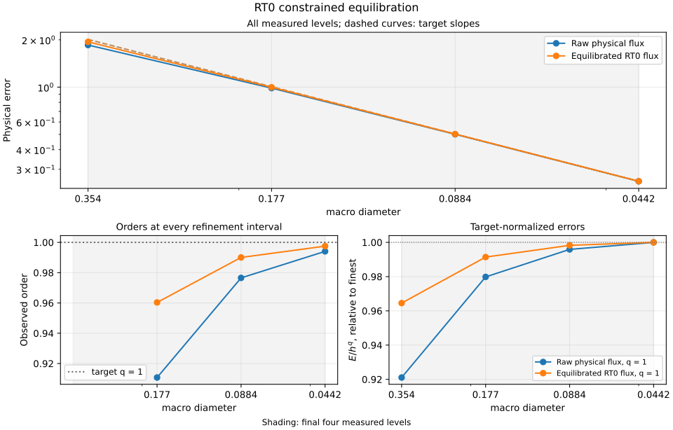
The constrained RT0 flux has consecutive observed orders 0.96034, 0.99005 and 0.99751. The normalized first-order amplitude has max/min ratio 1.03677. These order-one approximation controls concern the distinct P3/P0/RT0 workflow and are not assigned the published RT2 reconstruction theorem.
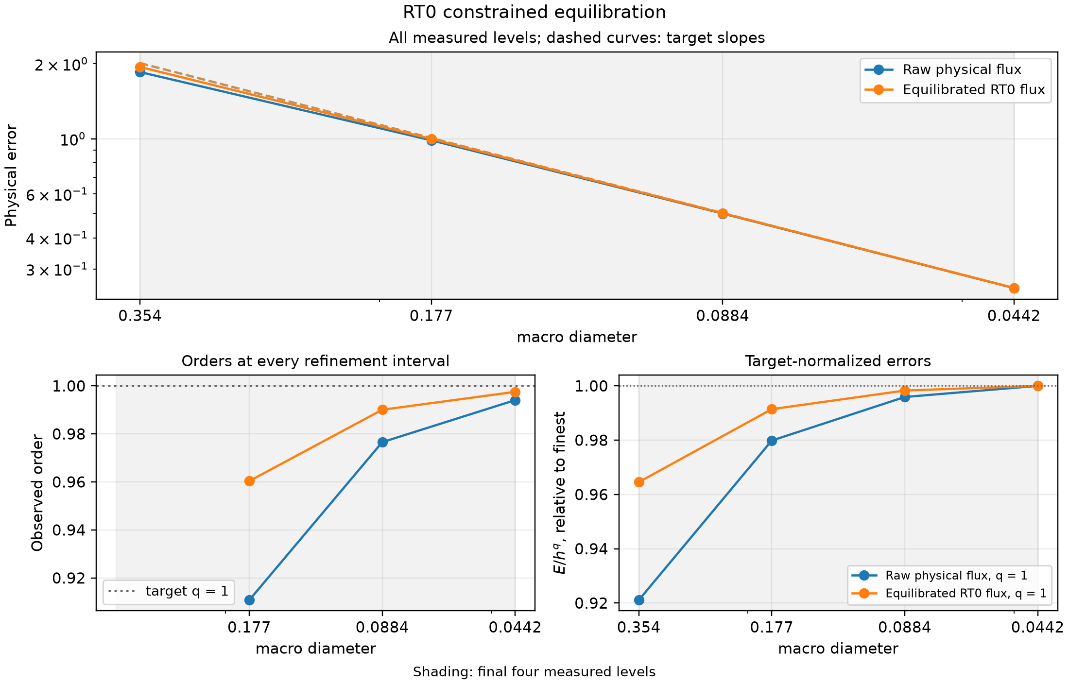
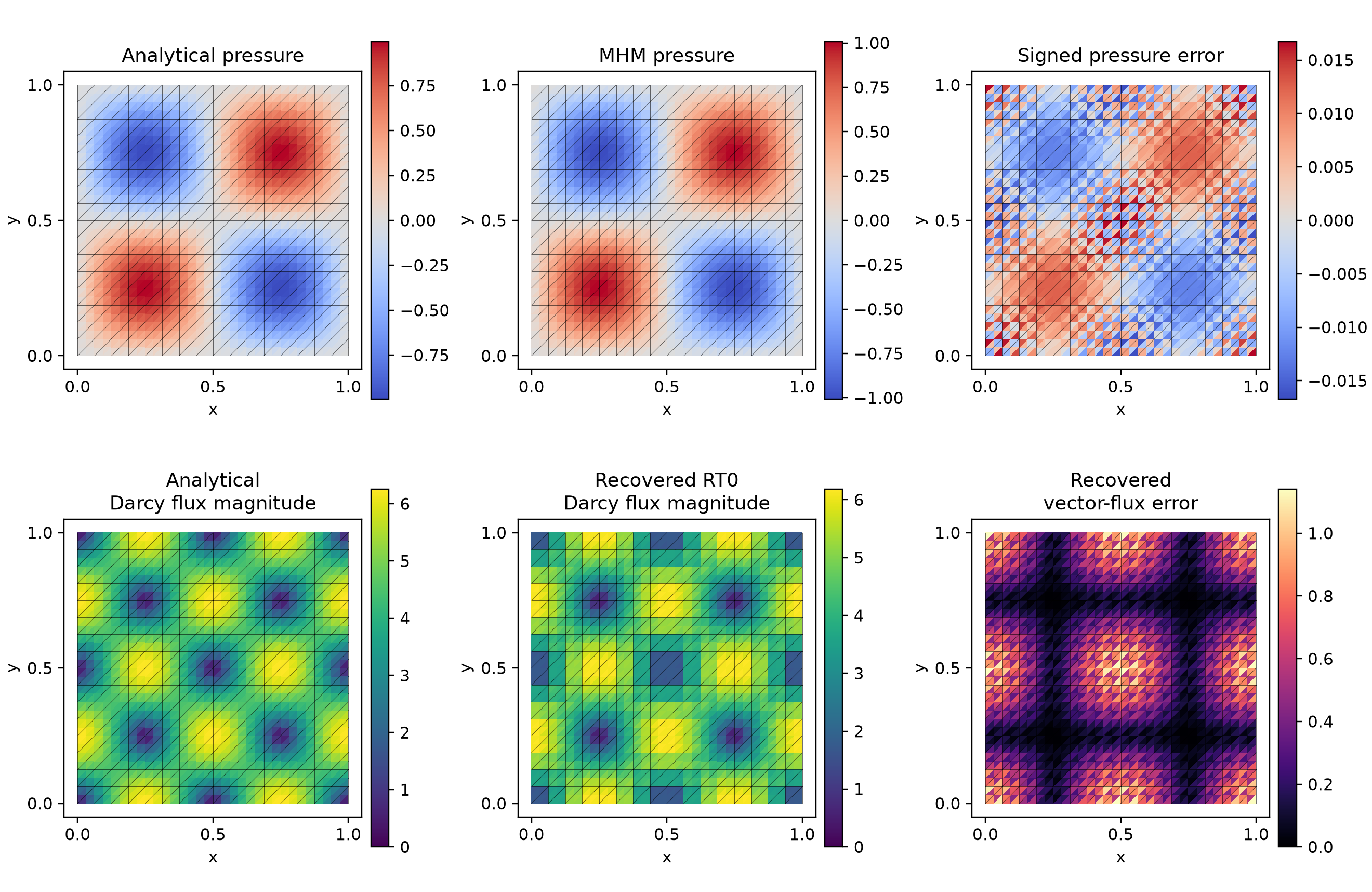
The RT0 panels use 512 actual macrotriangles and independent one-sided fine-cell centroid samples. Strict integrated fine-cell balance, H(div) conformity and physical approximation error are separate properties.
The indicator lesson evaluates reliability and convergence of the estimator; the adaptive lesson uses it on a localized smooth solution.
Reproduce this tutorial
The notebook linked at the top defines the forms and runs the recovery, indicator, adaptive and recursive studies. Install the native notebook backend as described in the installation guide, then open it from the source checkout:
References
- Gabriel R. Barrenechea, Larissa Martins, Weslley Pereira and Frédéric Valentin (2026). An H(div; Ω)-Conforming Flux Reconstruction for the Multiscale Hybrid-Mixed Method, Multiscale Modeling & Simulation 24(2), 399–428. DOI: 10.1137/24M1673073; accepted author manuscript.
- Christopher Harder, Diego Paredes and Frédéric Valentin (2013). A family of Multiscale Hybrid-Mixed finite element methods for the Darcy equation with rough coefficients, Journal of Computational Physics 245, 107–130. DOI: 10.1016/j.jcp.2013.03.019.