Darcy flow through an SPE10 reservoir layer

Connected channels and low-permeability barriers determine flow through the complete horizontal layer 36 of SPE10 Model 2. The input retains all \(60\times220\) material pixels, including both \(K_{xx}\) and \(K_{yy}\), without cropping or contrast clipping. In this layer the two components are equal.

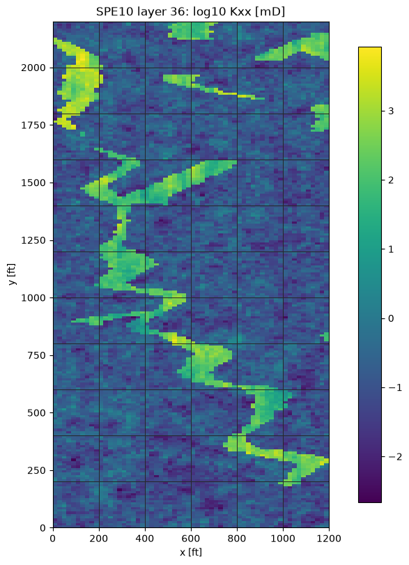
Logarithmic SPE10 layer-36 permeability and the actual macro mesh

The image shows \(\log_{10}(K_{xx}/\mathrm{mD})\), a prescribed material coefficient. Pressure and Darcy flux are computed solution fields and are shown in the results below.

Physical problem

Coordinates use the benchmark's feet convention and permeability is in mD. Pressure has a prescribed dimensionless difference of one:

\[ \begin{aligned} \Omega&=(0,1200)\times(0,2200),\\ \boldsymbol q&=-K\nabla p, & \nabla\cdot\boldsymbol q&=0,\\ p(x,0)&=1, &p(x,2200)&=0,\\ \boldsymbol q\cdot\boldsymbol n&=0 &&\text{on the two vertical walls}. \end{aligned} \]

Uniformly converting permeability and lengths to SI preserves this pressure-driven Darcy pressure and changes the flux units. Porosity is not part of this steady single-phase pressure equation.

Multiscale formulation and implementation

The application uses a \(6\times11\) square macro mesh, continuous local \(Q_1\) pressure, and continuous piecewise \(P_1\) flux traces on 16 segments per macroface. Each local grid has \(80\times80\) quadrilaterals, fitted to the material pixels. The face orientation \(s_{TF}\) comes from bind_interface.

The local and global equations are, respectively,

\[ \begin{aligned} \int_T K\nabla p_T\cdot\nabla v +\langle s_{TF}\lambda,v\rangle_{\partial T}&=0,\\ -\sum_T\langle s_{TF}\mu,p_T\rangle_{\partial T} &=-\langle\mu,p_D\rangle_{\Gamma_D}. \end{aligned} \]

Here \(\lambda\) is the globally oriented physical normal Darcy flux; its coefficients are zero on the no-flow walls. Each local constant is retained, so its compatibility equation enforces macro conservation. The pressure boundary data remove the global constant ambiguity.

This excerpt shows the forms passed by the application's local provider; K is the unchanged tensor-valued DG0 material on the fitted native mesh:

a = ufl.inner(K * ufl.grad(p), ufl.grad(v)) * dx
load = f * v * dx
b = local.trace_pairings(lambda phi, ds: phi * v * ds)
c = local.trace_pairings(lambda phi, ds: -phi * p * ds, axis="rows")
local.field("pressure", binding)

The complete implementation defines the coefficient, local kernel and moments, boundary data, MeshHierarchy, global Equation, assembly and solution. The primal MHM tutorial explains the method independently of this reservoir application.

Results and reproducibility

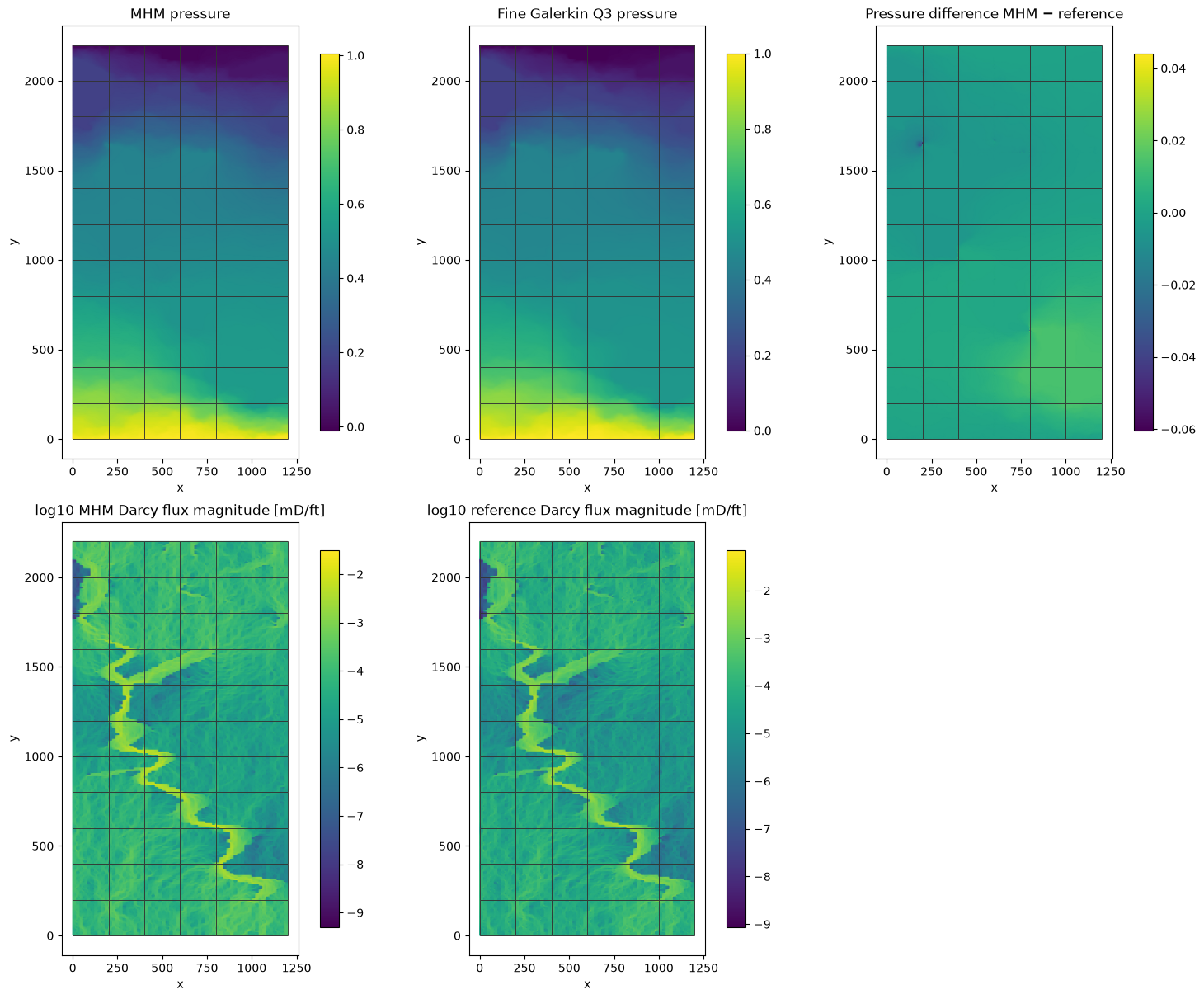
MHM and reference pressure and physical Darcy flux magnitude

Pressure decreases from the bottom to the top, with concentrated Darcy flux in conducting channels. The plotted volume flux is \(-K\nabla p_h\); it is a broken gradient reconstruction, rather than an H(div) field. Macro conservation does not assert conservation on every fine cell.

The notebook computes conforming pressure and flux comparisons and checks the reference's own refinement. It reports numerical differences, rather than an exact-solution error. A separate published-space reservoir study uses 32 trace segments and 120 local subdivisions; these distinct configurations are not mixed in one result.

Open the rendered application and its downloadable notebook. The material's revision, layer index, units and checksums accompany its companion archive. The local refinement is a declared choice; the source article does not specify that count.

References

Mike A. Christie and Martin J. Blunt (2001). Tenth SPE Comparative Solution Project: A Comparison of Upscaling Techniques. DOI: 10.2118/72469-PA.
Christopher Harder, Diego Paredes and Frédéric Valentin (2013). A family of Multiscale Hybrid-Mixed finite element methods for the Darcy equation with rough coefficients. DOI: 10.1016/j.jcp.2013.03.019.
Diego Paredes, Frédéric Valentin and Henrique M. Versieux (2024). Revisiting the robustness of the multiscale hybrid-mixed method: The face-based strategy. DOI: 10.1016/j.cam.2023.115415.