MH²M: pressure, conormal and shared trace
Open the step-by-step notebook · Download notebook
Follow the numbered steps: state the variational problem, choose the local and trace spaces, declare the local and global equations, solve, and inspect the physical fields.
The main workflow is meshes → spaces → local equations → global balance → assemble → solve → fields and errors. MeshHierarchy associates macro and local meshes; bind_interface and LocalContext own supported numbering, geometric orientation and native coordinate conversions. The mathematical forms, physical trace meaning, local modes and gauge remain explicit in the cells below. Fully manual/custom spaces use the same numerical owners; see the custom-interface notebook.
The three-field Multiscale Method (MH²M) uses local pressure, local boundary conormal and a shared global pressure trace. We declare all three equations explicitly and let LocalEquations and MultiscaleProblem eliminate the local fields.
Our two-dimensional P1/P0/P1 family follows de Barros, Madureira and Valentin (2026, version 3), equations (7), (28)–(29) and section 6.2. The oscillatory material and meshes below define an original introductory case, not a reproduction of the article's heterogeneous figures.
All problem data, boundary conditions, provider, classical baseline, reconstruction, norms and plots are defined in notebook cells. PyMHM supplies only generic finite-element and algebraic operations. Open the downloaded notebook in a writable directory:
Execution is serial; process workers need importable provider callables.
Field evaluation, norms, plots and executed-array archives use the importable supporting scalar helpers. The physical data and local/global variational equations remain explicit below.
The PyMHM distribution contains only the library. The first cell explicitly
downloads a checksum-verified companion archive and prepares the declared data
using its local Python helpers. You can inspect these support files in ROOT.
Complete studies and historical replay retain their existing opt-in flags.
from pathlib import Path
import os
import sys
from pymhm.io.workspace import workspace_from_archive

# Download verified support files; this operation does not execute them.
COMPANION_URL = "https://ipes-lncc.github.io/pymhm/downloads/35d2e7fcf53362a350d2f63714e035ebaac3c9388aeef7d0605955acc0154ea9/mh2m_multiscale-companion.zip"
COMPANION_SHA256 = "35d2e7fcf53362a350d2f63714e035ebaac3c9388aeef7d0605955acc0154ea9"
WORKSPACE = Path(
    os.environ.get("PYMHM_WORKSPACE", Path.cwd() / ".pymhm-companions" / COMPANION_SHA256)
)
ROOT = workspace_from_archive(COMPANION_URL, sha256=COMPANION_SHA256, directory=WORKSPACE)
os.environ["PYMHM_WORKSPACE"] = str(ROOT)
if str(ROOT) not in sys.path:
    sys.path.insert(0, str(ROOT))

# Explicitly prepare declared data with the downloaded Python helpers.
from scripts.notebook_reproduction import notebook_workspace

ROOT = notebook_workspace("introduction/mh2m_multiscale.ipynb", directory=ROOT)
root = ROOT
print("Workspace:", ROOT)


import numpy as np
import matplotlib.pyplot as plt
from typing import Any
from scipy import sparse
from threadpoolctl import threadpool_limits
from pymhm import Equation, LocalEquations, assemble
from pymhm import MeshHierarchy, LocalContext, bind_interface, bind_problem
from pymhm.core.equations import compile_form
from pymhm.fem.traces.interval import FaceSpace, SkeletonSpace
from examples.introduction.scalar import (
    plot_material,
    plot_reference_differences,
    plot_scalar_comparison,
    executed_array_digest,
    ScalarField,
    archive_cell,
    compare_scalar_fields,
    dirichlet_solve,
    native_scalar_space,
    save_scalar_report,
)
from pymhm.fem.scalar.triangle import nodal_space
from pymhm.meshes.triangle import TriangleMesh
from pymhm.backends.forms import assemble_pairing

plt.rcParams.update({"figure.dpi": 110, "font.size": 10})
from pymhm import solve
from pymhm.fem.traces.pressure_2d import PressureTraceSpace
1. The physical problem and the conormal sign
Use the same scalar Darcy problem as the MsHHO introduction:
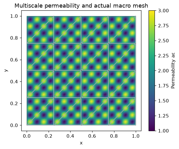
The article's conormal \(\eta_K\) has the opposite sign to physical outward flux. Each macrocell has its private copy on a shared face; pressure trace \(\rho\) is global. The coefficient has ellipticity bounds 1 and 3.
Our 32 macrotriangles do not resolve eight oscillations per direction. Each local mesh has 16 subdivisions per macroedge, keeping the material inside assembly and physical flux norms. This is fine local resolution on a simple macro mesh, not replacement of the coefficient by its average.
epsilon = 1 / 8


def permeability(points: np.ndarray) -> np.ndarray:
    """Evaluate aε I through its positive scalar factor, with ε=1/8."""
    phase = 2 * np.pi * points / epsilon
    return 2 + np.sin(phase[:, 0]) * np.sin(phase[:, 1])


macro = TriangleMesh.unit_square(4)
source = 1.0
local_refinement = 16
assembly_order = 8
print(
    {
        "macro_triangles": len(macro.cells),
        "epsilon": epsilon,
        "H_max": float(macro.lengths.max()),
        "h_max": float(macro.lengths.max() / local_refinement),
        "ellipticity_bounds": [1.0, 3.0],
        "source": source,
    }
)
{'macro_triangles': 32, 'epsilon': 0.125, 'H_max': 0.3535533905932738, 'h_max': 0.02209708691207961, 'ellipticity_bounds': [1.0, 3.0], 'source': 1.0}
2. Choose compatible spaces before assembling operators
Use \(k=0\) in the two-dimensional family of section 6.2:
Each pressure segment contains two conormal segments (M2), and each conormal segment contains two local boundary edges (M1). The uniform partitions match between incident macrocells. These mesh conditions accompany the chosen degrees; matrix dimensions alone do not establish compatibility.
PressureTraceSpace shares pressure values at macrovertices and numbers interior face nodes. SkeletonSpace supplies the broken conormal basis, with a private copy per macrocell. Only gamma coordinates are global.
local_degree = 1
gamma_segments, conormal_segments = 4, 8
gamma = PressureTraceSpace.uniform(macro, degree=1, segments=gamma_segments)
conormal = SkeletonSpace(
    macro,
    tuple(FaceSpace.uniform(0, conormal_segments) for _ in macro.faces),
)
assert conormal_segments == 2 * gamma_segments
assert local_refinement == 2 * conormal_segments
pressure_interface = bind_interface(gamma, convention="value")
conormal_interface = bind_interface(conormal, convention="value")
print(
    {
        "global_pressure_trace_coordinates": gamma.size,
        "local_conormal_unknowns_per_macrocell": 3 * conormal_segments,
        "local_P1_nodes_per_macrocell": (local_refinement + 1) * (local_refinement + 2) // 2,
    }
)
{'global_pressure_trace_coordinates': 193, 'local_conormal_unknowns_per_macrocell': 24, 'local_P1_nodes_per_macrocell': 153}
3. Write the three variational equations
For each macrocell \(K\),
The second equation matches trace moments against P0; it does not impose pointwise equality. The third equation balances conormal against continuous pressure trace tests.
With \(A_{ij}=a_K(\phi_j,\phi_i)\), \(B_{ij}=\int_{\partial K}\phi_i\mu_j\) and \(P_{j\ell}=\int_{\partial K}\mu_j\psi_\ell\),
Write the boundary pairing \(B\) as phi * v * ds in UFL, selecting the private conormal space as its interface. local.interface_pairing(conormal_interface) integrates \(P\) on the union of the pressure and conormal partitions and accumulates shared pressure vertices. Both are unsigned local boundary pairings: their mathematical signs are the explicit \(-B\) and \(-B^T\) in the saddle. The context owns face ordering and coefficient transport.
Write the local differential operator in UFL
Define the trial pressure p and test pressure v on the local Pk space. The UFL expressions below are the executable weak form, mass pairing and source. Changing this expression defines a new local operator; the multiscale contracts do not select a physical model.
local.native_space binds the declared fine mesh and equispaced element. The local saddle keeps its native pressure coordinates; compile_form assembles the expressions and releases native assembly resources. The same weak form can return portable nodal matrices for the independent classical baseline. The following section declares the two boundary spaces and their pairings.
import basix.ufl
import ufl


def user_volume_forms(
    fine: TriangleMesh,
    degree: int,
    *,
    binding: Any = None,
    portable: bool = True,
) -> tuple[Any, Any, np.ndarray]:
    """Assemble the user weak form in native or declared portable nodal coordinates."""
    if binding is None:
        _, V, order = native_scalar_space(fine, degree)
    else:
        V, order = binding.space, binding.mapping
    p, v = ufl.TrialFunction(V), ufl.TestFunction(V)
    x = ufl.SpatialCoordinate(V.mesh)
    a_epsilon = 2 + ufl.sin(2 * np.pi * x[0] / epsilon) * ufl.sin(2 * np.pi * x[1] / epsilon)
    dx = ufl.Measure("dx", domain=V.mesh, metadata={"quadrature_degree": 2 * assembly_order})
    a = a_epsilon * ufl.inner(ufl.grad(p), ufl.grad(v)) * dx
    mass = p * v * dx
    L = source * v * dx
    A, M, F = compile_form(a), compile_form(mass), compile_form(L)
    if portable:
        return A[order][:, order].tocsc(), M[order][:, order].tocsc(), F[order]
    return A, M, F
first_fine = macro.submesh(0, local_refinement)
A_ufl, M_ufl, F_ufl = user_volume_forms(first_fine, local_degree)
print(
    {
        "operator": "user-written UFL",
        "local_nodal_unknowns": A_ufl.shape[0],
        "constant_kernel_relative": float(
            np.linalg.norm(A_ufl @ np.ones(A_ufl.shape[0])) / sparse.linalg.norm(A_ufl)
        ),
    }
)
form_equivalence = {}  # Filled by the optional convenience check at the end.
{'operator': 'user-written UFL', 'local_nodal_unknowns': 153, 'constant_kernel_relative': 1.3562500818233753e-16}
def local_three_field_equations(local: LocalContext) -> LocalEquations:
    """Declare native pressure/conormal equations and the shared pressure balance."""
    fine = local.mesh
    element = basix.ufl.element(
        "Lagrange",
        "triangle",
        local_degree,
        lagrange_variant=basix.LagrangeVariant.equispaced,
    )
    pressure_space = local.native_space(element)
    stiffness, mass, force = user_volume_forms(
        fine,
        local_degree,
        binding=pressure_space,
        portable=False,
    )
    v = ufl.TestFunction(pressure_space.space)
    boundary_forms = local.trace_pairings(
        lambda phi, ds: phi * v * ds,
        interface=conormal_interface,
    )
    B = assemble_pairing(boundary_forms.forms)
    P = local.interface_pairing(conormal_interface, order=4)

    # These block dimensions express the three-field formulation itself.
    npressure, nconormal = stiffness.shape[0], B.shape[1]
    local_saddle = sparse.bmat([[stiffness, -B], [-B.T, None]], format="csc")
    coupling = np.vstack((np.zeros((npressure, P.shape[1])), P))
    pressure_reconstruction = np.hstack((np.eye(npressure), np.zeros((npressure, nconormal))))
    local.field("pressure", pressure_space, reconstruction=pressure_reconstruction)
    return local.equations(
        a=local_saddle,
        L=np.r_[force, np.zeros(nconormal)],
        b=coupling,
        c=coupling.T,
        metadata={
            "mesh": fine,
            "A": stiffness,
            "F": force,
            "B": B,
            "P": P,
            "pressure_count": npressure,
            "volume_moments": np.asarray(mass.sum(axis=1)).ravel(),
        },
    )
4. Declare the shared trace equation and recover pressure
The stiffness \(A_K\) alone has a constant kernel. For the compatible spaces above, the complete local saddle is invertible: boundary pairings fix the constant and trace moments. We neither invent a kernel for that saddle nor pin an arbitrary pressure node.
The local unknown of LocalEquations is \((p_K,\eta_K)\). The coupling b is \([0;P]\), and the global balance c is its transpose. Generic assembly eliminates both local fields, leaving \(\rho\). Dirichlet fixes its exterior nodes, so no global pressure gauge remains.
The article's Neumann maps use a boundary-mean-zero decomposition. The full saddle below retains the complete pressure and does not select any nodal or volume-mean complement. It expresses the same three-field equations directly. The field record below associates the pressure coefficients with their executed P1 basis; it contains no formulation or solver.
hierarchy = MeshHierarchy(
    macro, tuple(macro.submesh(cell, local_refinement) for cell in range(len(macro.cells)))
)
problem = bind_problem(
    hierarchy,
    pressure_interface,
    local_three_field_equations,
    global_equation=Equation(0, 0),
    retained=0,
    fixed=lambda global_context: global_context.fix_faces(macro.boundary_faces, 0),
)
with threadpool_limits(1):
    system = assemble(problem)
    solution = solve(system)
pressure_fields = solution.field("pressure")
physical_fields = tuple(
    ScalarField(field.mesh, local_degree, field.portable_coefficients) for field in pressure_fields
)
global_free_unknowns = gamma.size - len(problem.fixed)
conormal_fields = tuple(
    mixed[data["pressure_count"] :]
    for data, mixed in zip(system.local_metadata, solution.fields, strict=True)
)
print({"global_pressure_trace_free": global_free_unknowns, "global_residual": solution.residual})
5. Check injectivity, trace moments and macro conservation
The constant test \(v=1\) gives
Thus physical outward flux \(q\cdot n_K=-\eta_K\) conserves on each macrocell. Check this balance, \(B^Tp_K=P\rho_K\), the constant stiffness kernel and the original pressure equation. A rank check on \(B\) confirms that no conormal mode is invisible on the first cell.
These are execution diagnostics. Uniform stability depends on the compatible spaces and M1/M2 conditions, not merely a small algebraic residual. Raw \(-a_\varepsilon\nabla p_h\) need not equal \(-\eta_K\) pointwise on a boundary and is not claimed to be an \(H(\mathrm{div})\) field on the fine mesh.
The physical reconstruction reads solution.local_trace(cell): the bound space supplies the executed local face coefficients, including any declared basis changes. The value convention used here has no outward-normal sign. The method's reconstruction matrix remains an explicit part of its mathematical definition.
diagnostics = {
    "constant_kernel_relative": 0.0,
    "trace_moment_max": 0.0,
    "macro_conservation_max": 0.0,
    "original_local_relative_residual": 0.0,
}
basis_digests = []
archive = {
    "macro_points": macro.points,
    "macro_cells": macro.cells,
    "pressure_trace": solution.trace,
    "gamma_nodes": gamma.nodes,
}
for cell, (data, field, eta) in enumerate(
    zip(system.local_metadata, physical_fields, conormal_fields, strict=True)
):
    A, F, B, P = data["A"], data["F"], data["B"], data["P"]
    executed_pressure = pressure_fields[cell].coefficients
    rho = solution.local_trace(cell)
    diagnostics["constant_kernel_relative"] = max(
        diagnostics["constant_kernel_relative"],
        float(np.linalg.norm(A @ np.ones(A.shape[0])) / np.linalg.norm(A.data)),
    )
    diagnostics["trace_moment_max"] = max(
        diagnostics["trace_moment_max"],
        float(np.max(abs(B.T @ executed_pressure - P @ rho))),
    )
    diagnostics["macro_conservation_max"] = max(
        diagnostics["macro_conservation_max"],
        float(abs(B.sum(axis=0) @ eta + F.sum())),
    )
    defect = A @ executed_pressure - B @ eta - F
    scale = max(np.linalg.norm(F), np.linalg.norm(A @ executed_pressure), np.linalg.norm(B @ eta))
    diagnostics["original_local_relative_residual"] = max(
        diagnostics["original_local_relative_residual"],
        float(np.linalg.norm(defect) / scale),
    )
    basis_digests.append(executed_array_digest(B, P))
    descriptor = pressure_fields[cell].definition.descriptor
    binding = solution.trace_bindings[cell]
    archive_cell(
        archive,
        cell,
        field,
        executed=pressure_fields[cell],
        trace_binding=binding,
        conormal=eta,
        boundary_pairing=B,
        pressure_trace_pairing=P,
    )
assert np.linalg.matrix_rank(system.local_metadata[0]["B"]) == 3 * conormal_segments
assert max(diagnostics.values()) < 1e-10
print(diagnostics)
{'constant_kernel_relative': 2.1836088566646393e-16, 'trace_moment_max': 4.336808689942018e-19, 'macro_conservation_max': 1.0443035325380379e-15, 'original_local_relative_residual': 7.692601965273089e-14}
6. A classical primal Galerkin baseline, with its own refinement check
On a fine globally conforming mesh, the baseline solves the same operator, material, source and boundary conditions:
Use P2 on 32, 64 and 128 squares per direction, each split into two triangles. Assembly and boundary identification are visible below; solve_linear owns the free algebraic solve. This classical global assembly is separate from multiscale condensation. Both use DOLFINx/UFL with the same weak form; their global assembly procedures and boundary spaces are separate.
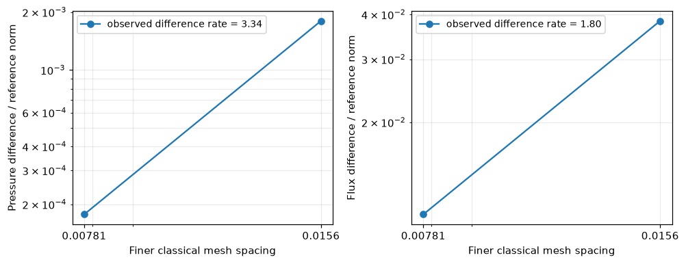
The finest classical field is a numerical reference, not an exact solution. First compare 32→64 and 64→128 in physical norms. The plotted difference rate is a reference-resolution indicator; two consecutive differences do not constitute a rigorous reference-error bound.
references = []
reference_dimensions = []
for resolution in (32, 64, 128):
    fine_global = TriangleMesh.unit_square(resolution)
    A_ref, _, F_ref = user_volume_forms(fine_global, 2)
    _, xy = nodal_space(fine_global, 2)
    boundary = np.flatnonzero(np.any(np.isclose(xy, 0) | np.isclose(xy, 1), axis=1))
    p_ref = dirichlet_solve(A_ref, F_ref, boundary, np.zeros(len(boundary)))
    references.append(ScalarField(fine_global, 2, p_ref))
    reference_dimensions.append(
        {
            "squares_per_direction": resolution,
            "triangles": len(fine_global.cells),
            "free_unknowns": len(p_ref) - len(boundary),
        }
    )
    print(reference_dimensions[-1])
reference = references[-1]
reference_refinement = [
    compare_scalar_fields((coarser,), finer, permeability, order=8)
    for coarser, finer in zip(references[:-1], references[1:])
]
for interval, norms in zip(("32 → 64", "64 → 128"), reference_refinement):
    print(interval, norms)

# These rates concern differences between successive reference meshes.
# They are indicators, not exact-solution error rates.
refinement_figure = plot_reference_differences(
    [1 / 64, 1 / 128],
    reference_refinement,
)

plt.show()

# A reference must resolve its own physical fields before serving as a baseline.
assert reference_refinement[-1]["pressure_relative"] < reference_refinement[0]["pressure_relative"]
assert reference_refinement[-1]["flux_relative"] < reference_refinement[0]["flux_relative"]
32 → 64 {'pressure_L2': 3.823696684608936e-05, 'flux_L2': 0.0073346478106178165, 'flux_energy': 0.005272480435871399, 'pressure_relative': 0.0018001151790877515, 'flux_relative': 0.03838323140026158, 'energy_relative': 0.03921980440020735}
64 → 128 {'pressure_L2': 3.7669518113256023e-06, 'flux_L2': 0.0021132796164602475, 'flux_energy': 0.0015405697662049793, 'pressure_relative': 0.00017731712073356501, 'flux_relative': 0.011059633117206041, 'energy_relative': 0.011458909837941546}
7. Compare pressure and physical flux on a common fine partition
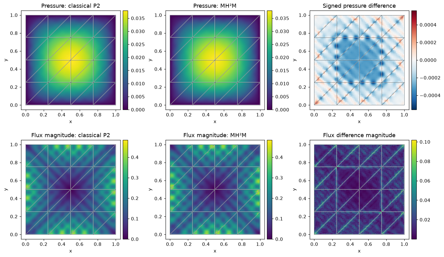
The reference mesh resolves every local mesh interface in this nested, uniformly refined case. Integrate on its triangles and use its field norms as denominators:
The comparison code keeps the coefficient inside flux and energy norms. Quadrature orders 8 and 10 independently check norm integration. At volume quadrature points, evaluate the original coefficients directly; do not compare images or interpolated color maps.
For plotting, sample every fine triangle separately. Duplicate interface points retain separate incident values. Pressure and flux-magnitude panels share scales with their reference panels; each difference has its own colorbar. All panels show the actual macro mesh.
errors_q8 = compare_scalar_fields(physical_fields, reference, permeability, order=8)
errors_q10 = compare_scalar_fields(physical_fields, reference, permeability, order=10)
quadrature_difference = max(
    abs(errors_q8[key] - errors_q10[key]) / max(abs(errors_q10[key]), np.finfo(float).tiny)
    for key in ("pressure_L2", "flux_L2", "flux_energy")
)
print(
    {"physical_relative_errors": errors_q10, "relative_norm_change_q8_q10": quadrature_difference}
)
assert quadrature_difference < 1e-5

figure = plot_scalar_comparison(
    macro,
    physical_fields,
    reference,
    permeability,
    numerical_label="MH²M",
)
plt.show()
{'physical_relative_errors': {'pressure_L2': 0.00019495407271239985, 'flux_L2': 0.01944959190409417, 'flux_energy': 0.013412679562910609, 'pressure_relative': 0.009176834899961196, 'flux_relative': 0.10178745352163324, 'energy_relative': 0.0997648332247903}, 'relative_norm_change_q8_q10': 1.9464623390029375e-15}
Optional: use a prepared operator for this weak form
For the scalar diffusion form written above, scalar_operators provides a
portable Basix assembly convenience. Defining a new physical operator does not
require this function: the main computation already assembles the UFL expression
written by the user. The following check verifies agreement in the same local
finite-element space and basis before substituting this convenience.
from pymhm.fem.scalar.triangle import scalar_operators

A_prepared, M_prepared, F_prepared = scalar_operators(
    first_fine,
    local_degree,
    diffusion=permeability,
    source=source,
    order=assembly_order,
)
form_equivalence = {
    "stiffness_relative": float(
        sparse.linalg.norm(A_ufl - A_prepared) / sparse.linalg.norm(A_prepared)
    ),
    "mass_relative": float(sparse.linalg.norm(M_ufl - M_prepared) / sparse.linalg.norm(M_prepared)),
    "source_relative": float(np.linalg.norm(F_ufl - F_prepared) / np.linalg.norm(F_prepared)),
}
assert max(form_equivalence.values()) < 1e-10
print(form_equivalence)
{'stiffness_relative': 2.681979681896503e-16, 'mass_relative': 6.514095339453426e-16, 'source_relative': 4.464810611149017e-16}
record = {
    "method": "MH²M",
    "physical_problem": f"-div(aε grad(p))={source:g}, p|boundary=0",
    "source": float(source),
    "epsilon": epsilon,
    "macro_triangles": len(macro.cells),
    "local_refinement": local_refinement,
    "local_degree": local_degree,
    "assembly_order": assembly_order,
    "error_orders": [8, 10],
    "global_free_unknowns": global_free_unknowns,
    "reference_dimensions": reference_dimensions,
    "reference_refinement": reference_refinement,
    "physical_errors": errors_q10,
    "quadrature_relative_difference": quadrature_difference,
    "global_residual": solution.residual,
    "diagnostics": diagnostics,
    "basis_digests": basis_digests,
    "form_equivalence": form_equivalence,
}
print(
    save_scalar_report(
        ROOT,
        "mh2m_multiscale",
        record,
        archive,
        {
            "physical-fields": figure,
            "permeability": fig_material,
            "reference-refinement": refinement_figure,
        },
    )
)
./build/docs-restructure/final-workspaces/provenance-final-mh2m_multiscale-ce2f83522ad1/build/introduction/mh2m_multiscale
8. Verify a compatible smooth three-field family
The oscillatory material study above is distinct from this smooth convergence control. Use the polynomial data of section 8.1 in de Barros, Madureira and Valentin (2026, version 3) on the unit square:
Keep the three-field equations written above. Choose continuous \(\Gamma=P_2\) on one macroface segment, \(\Lambda=P_1\) on two segments and local P2 pressure with four edge subdivisions. Each pressure segment contains two conormal segments (M2), and each conormal segment contains two local edges (M1). These ratios remain fixed through \(n=2,4,8,16,32\).
Theorem 19 gives the second-order energy target under the two-dimensional M1/M2 Fortin conditions, regular aligned partitions and the stated pressure, source-lift and volume-flux regularity. Third-order pressure is observed separately. The paper's coarser section-8.1 P2/P1/P2 experiment, with one Lambda segment and two local subdivisions, does not satisfy M2 and is discussed in Remark 16; it is not substituted for this compatible family. A small residual alone does not justify transferring the estimate to that coarser configuration or to a different material or domain.
The local pressure equation, pressure/conormal pairing and free Gamma balance are checked in their original coefficient coordinates, separately from physical-error integration.
Recompute every measured order
For successive physical errors \(E_{i-1},E_i\) at the actual macro diameters, compute
The cell reads the attributed numerical record, displays every measured level and recomputes its orders. It does not execute a PDE acquisition. The fitted terminal slope uses the final four levels and their three intervals. For each declared target \(q\), the amplitude ratio is the maximum divided by the minimum of \(E/H^q\) over those same levels. A value near one indicates stabilization of the compensated error; an observed L2 order is kept separate from a proved energy estimate.
import json
from IPython.display import Markdown, display
from examples.tutorial_convergence import refinement_series, asymptotic_summary, plot_method_series
refinement_record = ROOT / 'examples/results/tutorial-methods/mh2m-compatible-current.json'
refinement_data = json.loads(refinement_record.read_text(encoding='utf-8'))
refinement_rows = refinement_data['rows']
refinement_error_keys = {'pressure L2': 'pressure_l2', 'broken gradient L2': 'gradient_l2'}
refinement_targets = {'broken gradient L2': 2.0}
refinement_rows = sorted(refinement_rows, key=lambda refinement_row: refinement_row['macro_diameter'], reverse=True)
refinement_sizes = np.asarray([refinement_row['macro_diameter'] for refinement_row in refinement_rows])
refinement_field_errors = {refinement_field: np.asarray([refinement_row[refinement_key] for refinement_row in refinement_rows]) for refinement_field, refinement_key in refinement_error_keys.items()}
refinement_orders = {refinement_field: np.log(refinement_values[:-1] / refinement_values[1:]) / np.log(refinement_sizes[:-1] / refinement_sizes[1:]) for refinement_field, refinement_values in refinement_field_errors.items()}
refinement_header = ['Refinement size'] + [refinement_column for refinement_field in refinement_error_keys for refinement_column in (refinement_field, 'Order')]
refinement_lines = [' | '.join(refinement_header), ' | '.join(['---'] * len(refinement_header))]
for refinement_index, refinement_size in enumerate(refinement_sizes):
    refinement_values = [f'{refinement_size:.6g}']
    for refinement_field in refinement_error_keys:
        refinement_values.extend([f'{refinement_field_errors[refinement_field][refinement_index]:.6e}', '—' if refinement_index == 0 else f'{refinement_orders[refinement_field][refinement_index - 1]:.3f}'])
    refinement_lines.append(' | '.join(refinement_values))
display(Markdown('\n'.join(refinement_lines)))
refinement_series_data = refinement_series(refinement_record, refinement_rows, 'macro_diameter', refinement_error_keys, refinement_targets, method='mh2m', spaces='Gamma P2, one segment; Lambda P1, two segments; local P2/r4; M1=M2=2', rate_provenance='de Barros, Madureira and Valentin (2026), version 3, Theorem 19: energy order two under the two-dimensional M1/M2 Fortin conditions, regular aligned partitions and the stated pressure/source-lift/volume-flux regularity; pressure order three observed separately.', root=ROOT)
print({'record': refinement_series_data['record'], 'sha256': refinement_series_data['sha256']})
for refinement_field, refinement_summary in asymptotic_summary(refinement_series_data).items():
    print(refinement_field, {'last_three_orders': [round(refinement_order, 3) for refinement_order in refinement_summary['orders']], 'fitted_order': round(refinement_summary['fitted_order'], 3), 'target': refinement_summary['target'], 'normalized_amplitude_ratio': refinement_summary.get('amplitude_ratio')})
plot_method_series(refinement_series_data)
plt.show()
| Refinement size | pressure L2 | Order | broken gradient L2 | Order |
|---|---|---|---|---|
| 0.707107 | 1.484152e-03 | — | 2.405119e-02 | — |
| 0.353553 | 1.907832e-04 | 2.960 | 6.968576e-03 | 1.787 |
| 0.176777 | 2.404196e-05 | 2.988 | 1.828945e-03 | 1.930 |
| 0.0883883 | 3.020023e-06 | 2.993 | 4.639316e-04 | 1.979 |
| 0.0441942 | 3.782056e-07 | 2.997 | 1.164489e-04 | 1.994 |
{'record': 'examples/results/tutorial-methods/mh2m-compatible-current.json', 'sha256': '5b8d1d24620542d6fba18a991badfe3b37fa2f28fa497d599e600d3070747556'}
pressure L2 {'last_three_orders': [2.988, 2.993, 2.997], 'fitted_order': 2.993, 'target': None, 'normalized_amplitude_ratio': None}
broken gradient L2 {'last_three_orders': [1.93, 1.979, 1.994], 'fitted_order': 1.969, 'target': 2.0, 'normalized_amplitude_ratio': 1.0694762344273008}
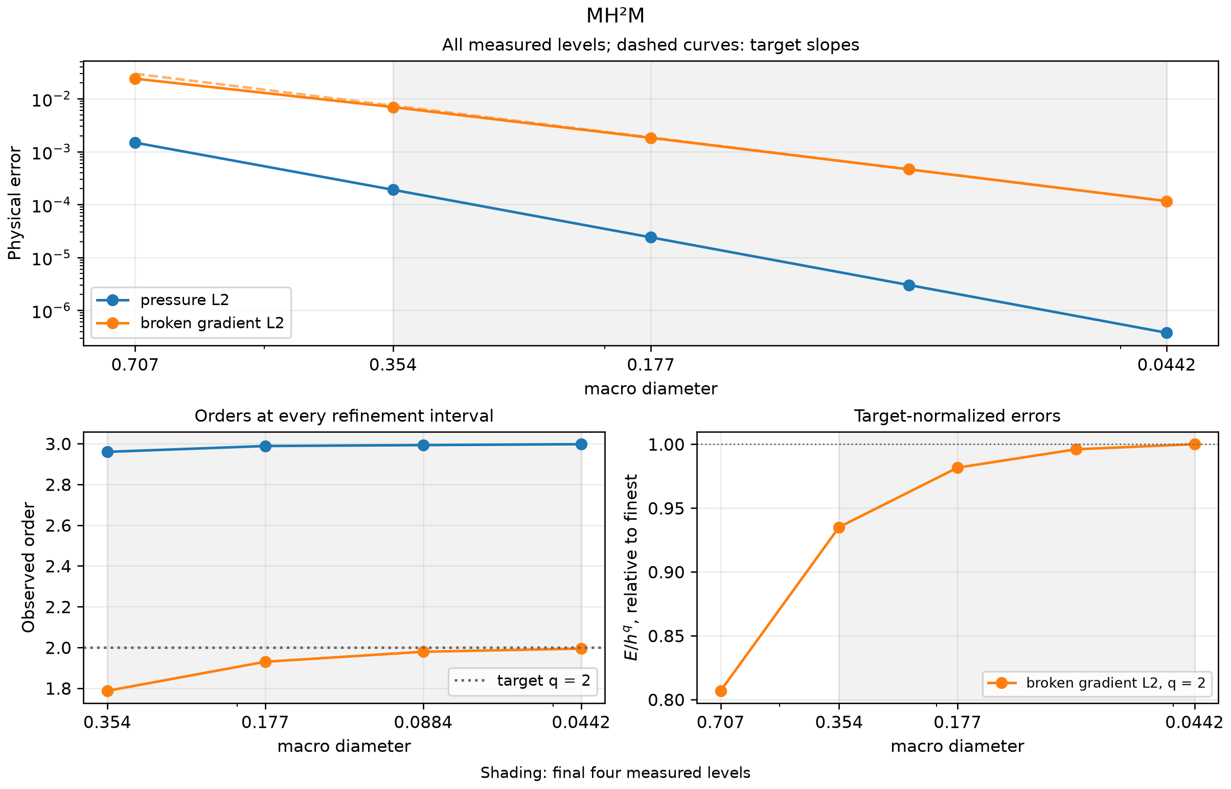
Download the figure as SVG or PDF. Shading covers the same final four levels in every panel; dashed curves are target powers anchored to the finest measured error.
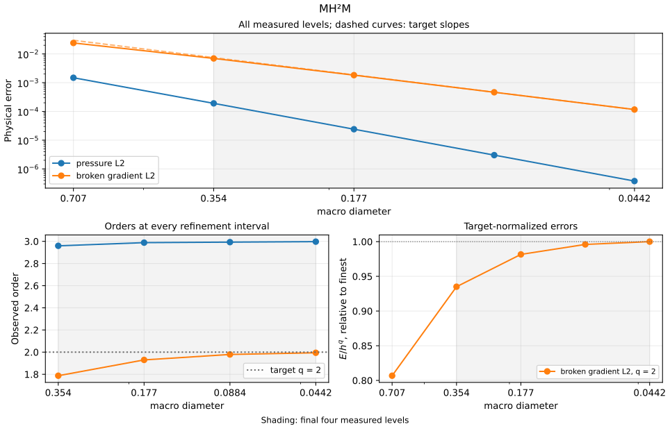
The current acquisition compares full physical norms at error quadrature orders 10 and 12; the largest relative difference over all levels and fields is 6.672e-14. It also checks the original method equations in their declared coefficient coordinates, retaining global compatibility, local reconstruction and physical field errors as separate quantities. Its source closure is unchanged during execution. The norm-only record contains no persisted coefficient vector.
Local Galerkin sensitivity at fixed macro resolution
Hold \(n=8\), the physical data and all trace spaces fixed, and double only the local subdivisions from 4 to 8. Pairwise differences are integrated on the nested finer partition using the executed coefficient bases. Discontinuous pressure and independent interface values remain separate. Both solutions are also compared directly with the analytical fields:
| Field | Coarse error | Refined error | Field difference | Difference / coarse error |
|---|---|---|---|---|
| pressure L2 | 2.404196e-05 | 2.385727e-05 | 5.385851e-07 | 2.240e-02 |
| broken gradient L2 | 1.828945e-03 | 1.826071e-03 | 1.107973e-04 | 6.058e-02 |
The r4/r8 comparison retains Gamma P2 on one segment and Lambda P1 on two segments. M2 is unchanged; the number of fine edges per Lambda segment rises from two to four, strengthening M1. Thus the local control compares two admissible realizations rather than replacing the pressure/flux trace spaces to improve the measured order.
The full physical-error norms agree at quadrature orders 10 and 12, with maximum relative change 1.199e-14. For the two-grid sensitivity, the change in the integrated field difference divided by the coarse analytical error is 4.422e-15. This scale assesses the local contribution to that physical error and remains meaningful when the two fields differ only at roundoff. The raw differences at both quadrature orders and their unscaled relative changes remain in the local-control record (SHA256 8933c2e8c4f68a626276c4a0fc8e1b06e14334f8f8c413a2649137de27fe2350). Original equations and reconstruction constraints retain their separate unchanged checks.
The smooth convergence figure uses the attributed numerical record (SHA256 5b8d1d24620542d6fba18a991badfe3b37fa2f28fa497d599e600d3070747556). The shared rate notebook compares the method sequences.
Reproduce this tutorial
View the source notebook or download the notebook, then open it:
The first cell downloads a SHA256-verified companion containing inspectable support files. Downloading does not execute them. Native UFL forms require the compatible backend described in the installation guide.
For batch execution, extract the same companion, change to its workspace and run:
The runner uses the active interpreter and writes an executed copy and receipt under build/notebooks/introduction/. Larger field archives have documented downloads.
Figures and outputs of sections 1–7 retain notebook SHA256 471d16e4f4e5bfa14e5933cfa8efce4a41996975b6115477935de8f565bfe953 in the publication manifest. The smooth convergence figure and tables use the separate numerical records cited in section 8. Running the current source produces a receipt for its actual notebook, support files and environment.
References
- Franklin de Barros, Alexandre L. Madureira, and Frédéric Valentin (2026). A three-field Multiscale Method. arXiv preprint, version 3, 5 August 2026; first submitted 25 April 2024. arXiv: 2404.16978v3.