Physical error indicators

Executable notebook · Download notebook

Use the already declared local/global UFL equations in the flux-recovery lesson, then measure the estimator alongside the true physical error. The smooth analytical case uses the same data as Barrenechea et al. (2026), §6.1. The study measures estimator decay and effectivity over a resolved refinement sequence; the reliability statement comes from the cited analysis under its stated hypotheses.

1. Solve the declared problem on compatible spaces

For \(\ell=0\) use P2 local pressure; for \(\ell=1\) use P3. The canonical reconstruction is RT2 in both branches, with \(h=H/2\). Identity diffusion, homogeneous Dirichlet pressure, convex macrotriangles and a globally conforming fine mesh are explicit inputs. They are hypotheses of the estimator, rather than automatically selected properties of a Darcy model.

with threadpool_limits(1):
    coefficients = solve(assemble(problem))
pressure_fields = coefficients.field("pressure")

The notebook constructs DarcySolution from these mapped coefficients and the independently defined source. No opaque problem-specific solver selects the physical formulation.

2. Form the four physical contributions

The estimator in equations (5.3)–(5.7) uses

\[ \begin{aligned} \eta_{1,T}&=\lVert\nabla p_h+q_h^R\rVert_{0,T},\\ \eta_{2,T}&=\lVert\nabla(p_h-I_{\mathrm{OS}}p_h)\rVert_{0,T},\\ \eta_{3,T}&=\frac{H_T}{\pi}\lVert\Pi_{T,2}\operatorname{div}q_h^R- \operatorname{div}q_h^R\rVert_{0,T},\\ \eta_{\mathrm{osc},T}&=\frac{H_T}{\pi}\lVert f-\Pi_{T,2}f\rVert_{0,T}. \end{aligned} \]

The conforming potential \(I_{\mathrm{OS}}p_h\) and the canonical RT2 flux \(q_h^R\) are separately reconstructed fields. Continuous-test equilibrium is checked before the reliability estimate is evaluated. Global original compatibility is a separate diagnostic; an independent volume/trace-row observer checks the local original equations on both degree branches.

estimate = estimate_darcy_error(
    solution, homogeneous_dirichlet=True, degree=2, quadrature_order=16,
)
energy_error = estimate.energy_error(exact_gradient, order=16)
assert max(estimate.equilibrium_defect) < 1e-10
assert estimate.total >= energy_error

3. Compare with the true error and inspect effectivity

Theorem 5.2 yields

\[ \begin{aligned} \lVert\nabla(p-p_h)\rVert_{0,\Omega}^2 &\le\sum_T\left[(\eta_{1,T}+\eta_{3,T}+\eta_{\mathrm{osc},T})^2 +\eta_{2,T}^2\right]=\eta^2,\\ I_{\mathrm{eff}}&=\frac{\eta}{\lVert\nabla(p-p_h)\rVert_{0,\Omega}}. \end{aligned} \]

The continuous theorem assumes exact integration. PyMHM reports positive quadrature estimates and checks a second independent error rule; it does not claim interval certification. An effectivity greater than one establishes the measured upper bound. Effectivity need not converge to one: its efficiency constant depends on the mesh ratio and approximation spaces.

4. Reach the smooth-case asymptotic regime

The current native study uses \(n=4,8,16,32\) square subdivisions, with every assembly and recovery recomputed. The broken energy error has order \(H^{\ell+1}\) under the stated regularity. For fixed \(H/h=2\), the estimator shows the same leading decay and stable effectivity; its individual contributions are plotted separately. This is the behavior illustrated by §6.1 of the paper; table ordinates are not asserted to be identical.

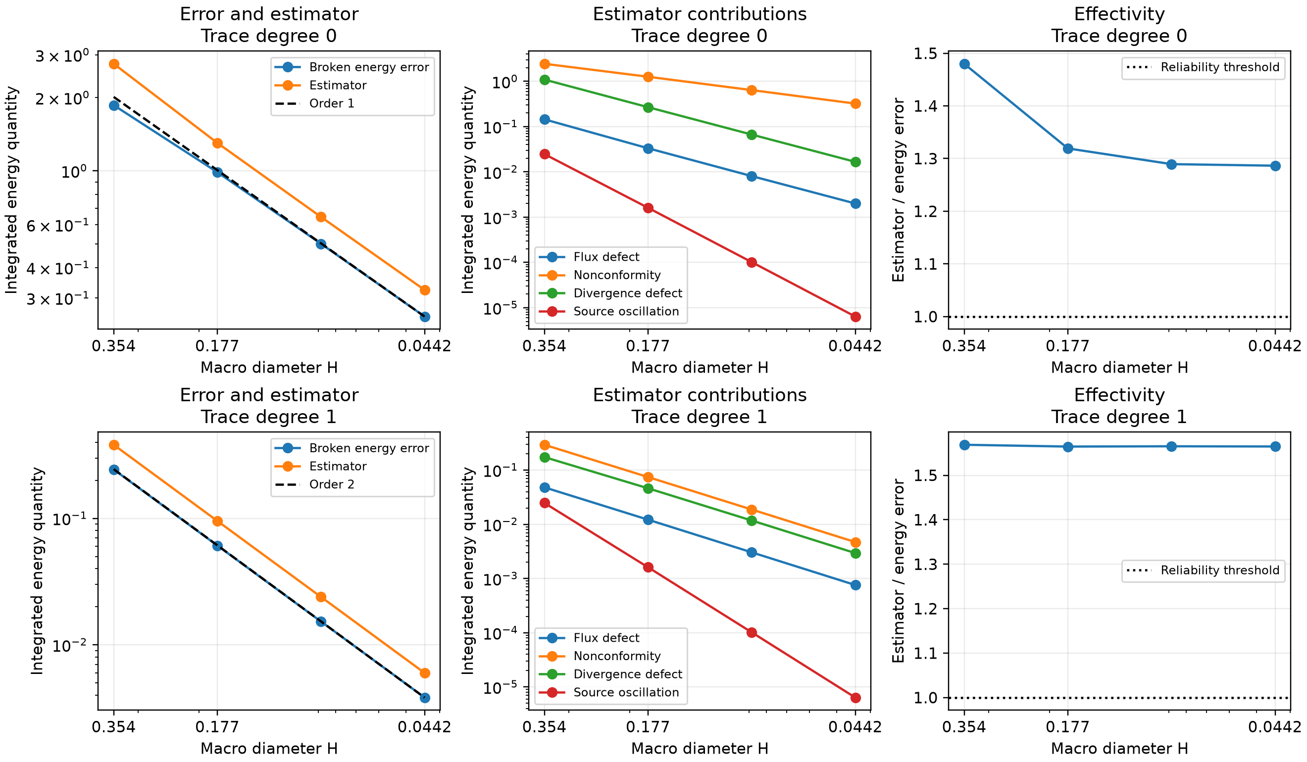
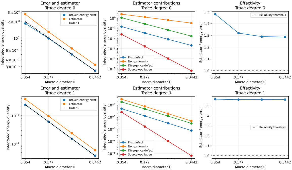
Estimator, individual contributions and effectivity on both trace-degree branches

PDF · SVG

Trace degree	Macro subdivisions	Broken energy error	Estimator	Effectivity
0	4	1.860873e+00	2.754206e+00	1.4801
0	8	9.865552e-01	1.301577e+00	1.3193
0	16	5.010100e-01	6.460385e-01	1.2895
0	32	2.514957e-01	3.235498e-01	1.2865
1	4	2.434897e-01	3.819492e-01	1.5686
1	8	6.097962e-02	9.540820e-02	1.5646
1	16	1.528115e-02	2.391859e-02	1.5652
1	32	3.826503e-03	5.987559e-03	1.5648

The independently assembled fine classical P3 baseline is checked against the same analytical pressure and physical flux on three refined global meshes. It is a numerical reference; the exact solution remains the analytical field.

The projected-divergence and source-oscillation contributions differ from Table 3 for the declared meshes. Exact historical macro/fine connectivity and executable estimator/projection inputs are unavailable, so the matching degree choices and decay rates do not establish reproduction of that table.

marked = mark_dorfler(estimate.local_squared, theta=0.5)
assert estimate.local_squared[marked].sum() >= 0.5*estimate.local_squared.sum()

local_squared contains integrated squared macro indicators. These values are not pointwise residual samples. Follow the adaptive workflow to rebuild the equations after marking and compare error against actual work.

Reproduce this tutorial

The notebook linked at the top defines the forms and runs the recovery, indicator, adaptive and recursive studies. Install the native notebook backend as described in the installation guide, then open it from the source checkout:

pixi run --locked -e introduction jupyter lab notebooks/darcy/reconstruction_and_indicators.ipynb

References

Gabriel R. Barrenechea, Larissa Martins, Weslley Pereira and Frédéric Valentin (2026). An H(div; Ω)-Conforming Flux Reconstruction for the Multiscale Hybrid-Mixed Method, Multiscale Modeling & Simulation 24(2), 399–428. DOI: 10.1137/24M1673073; accepted author manuscript.
Christopher Harder, Diego Paredes and Frédéric Valentin (2013). A family of Multiscale Hybrid-Mixed finite element methods for the Darcy equation with rough coefficients, Journal of Computational Physics 245, 107–130. DOI: 10.1016/j.jcp.2013.03.019.