Stokes–Brinkman MHM

Build mixed velocity–pressure UFL equations on local meshes, couple them through a vector pseudotraction trace, and impose one physical pressure gauge after assembly. This tutorial compares stable Taylor–Hood local Galerkin with the residual-stabilized equal-order MHM-USFEM variant.

Executable boundary-layer notebook · Download notebook

The notebook runs in introduction; it declares its exact data, local and reference UFL forms, global equation, physical norms and plotting workflow in successive cells. Convergence on the difficult layer is separated from the smooth asymptotic study at the end of this page.

1. Start with the PDE and analytical layer

Use the vector-Laplacian convention from Section 3.1.2 of Araya et al. (2017):

\[ \begin{aligned} -\nu\Delta u+\gamma u+\nabla p&=f, &\nabla\cdot u&=0,\\ u_*&=(y-g(y),x-g(x)), &p_*&=x-y,\\ g(s)&=\frac{e^{(s-1)/\nu}-e^{-1/\nu}}{1-e^{-1/\nu}}, &\nu&=10^{-2},\quad\gamma=1. \end{aligned} \]

The layer width is \(\nu\). Prescribe \(u_*\) on the entire exterior and set the physical pressure integral to zero. Differentiate these analytical functions to obtain the source, before constructing the discrete operator:

\[ f=\nu(g''(y),g''(x))+\gamma u_*+(1,-1). \]

denominator = -np.expm1(-1/NU)
x = ufl.SpatialCoordinate(domain)
g = lambda s: (ufl.exp((s-1)/NU)-np.exp(-1/NU))/denominator
truth_u = ufl.as_vector((x[1]-g(x[1]), x[0]-g(x[0])))
truth_p = x[0]-x[1]
force = (
    ufl.as_vector((ufl.exp((x[1]-1)/NU), ufl.exp((x[0]-1)/NU)))
    /(NU*denominator)+GAMMA*truth_u+ufl.as_vector((1.0, -1.0))
)

The source includes both resistance and the pressure gradient. An exponential layer that a local mesh does not resolve need not exhibit an asymptotic rate.

2. Choose macro, local and interface spaces

The Taylor–Hood comparison uses P2 velocity/P1 pressure with four subdivisions per macro edge, including an interior vertex in each local triangulation. Its equal-order comparison uses P2/P2 on the same local meshes. The vector trace uses P0 coordinates on complete macrofaces for this comparison.

macro = TriangleMesh.unit_square(n)
skeleton = SkeletonSpace(
    macro, tuple(FaceSpace.uniform(0) for _ in macro.faces), components=2,
)
hierarchy = MeshHierarchy(
    macro, tuple(macro.submesh(i, 4) for i in range(len(macro.cells))),
)
interface = bind_interface(skeleton, convention="normal")

The separate polynomial convergence family uses one local triangle per macrocell, unsplit P\(\ell\) traces and stabilized P\(_{\ell+2}\)/P\(_{\ell+2}\) local spaces, for \(\ell=0,1,2\). It satisfies the two-dimensional sufficient condition \(k-\ell\ge2\). These are distinct approximation families; their results must retain their own space descriptions. Araya et al. (2025) states the lifting, degree and regularity hypotheses.

3. Write the local momentum and incompressibility forms

For \(w=(u,p)\) and \(z=(v,q)\), the pressure test convention is

\[ B_K(w,z)=\nu(\nabla u,\nabla v)_K+\gamma(u,v)_K -(p,\nabla\cdot v)_K-(q,\nabla\cdot u)_K. \]

Use a Basix mixed element, then write this equation with UFL:

pressure_degree = velocity_degree if stabilized else velocity_degree-1
element = basix.ufl.mixed_element([
    basix.ufl.element("Lagrange", "triangle", velocity_degree, shape=(2,)),
    basix.ufl.element("Lagrange", "triangle", pressure_degree),
])
W = dolfinx.fem.functionspace(domain, element)
u, p = ufl.TrialFunctions(W)
v, q = ufl.TestFunctions(W)
dx = ufl.Measure("dx", domain=domain, metadata={"quadrature_degree": 28})
a = (
    NU*ufl.inner(ufl.grad(u), ufl.grad(v))+GAMMA*ufl.inner(u, v)
    -p*ufl.div(v)-q*ufl.div(u)
)*dx
L = ufl.inner(force, v)*dx
mean_form = q*dx

For USFEM, declare the complete momentum residual and include its matching source term:

\[ \begin{aligned} R(u,p)&=-\nu\Delta u+\gamma u+\nabla p,\\ B_K^{\mathrm{US}}(w,z)&=B_K(w,z)-\sum_{\tau\subset K} \kappa_\tau(R(w),R(z))_\tau,\\ F_K^{\mathrm{US}}(z)&=(f,v)_K-\sum_{\tau\subset K} \kappa_\tau(f,R(z))_\tau. \end{aligned} \]

R = -NU*ufl.div(ufl.grad(u))+GAMMA*u+ufl.grad(p)
Rtest = -NU*ufl.div(ufl.grad(v))+GAMMA*v+ufl.grad(q)
h = ufl.CellDiameter(domain)
tau = h**2/(ufl.max_value(GAMMA*h**2, 4*NU/inverse_m)+4*NU/inverse_m)
a -= tau*ufl.inner(R, Rtest)*dx
L -= tau*ufl.inner(force, Rtest)*dx

inverse_m is computed on the actual velocity polynomial space with laplacian_inverse_bound. The notebook displays the quotient and verifies its matrix inequality. Keeping only a pressure-gradient penalty would omit resistance and higher-order Laplacian terms from this method. The negative residual sign and stabilized load are essential.

4. Declare both interface actions

The local unknown is the oriented vector-Laplacian pseudotraction,

\[ \lambda_K=(-\nu\nabla u+pI)n_K. \]

This convention follows the grad–grad volume form. Symmetric Cauchy stress uses a different natural traction and kernel. Binding handles the incidence signs; the mathematical pairings remain visible:

binding = local.native_space(W)
u, p = ufl.TrialFunctions(W)
v, q = ufl.TestFunctions(W)
b = local.trace_pairings(lambda phi, ds: ufl.inner(phi, v)*ds)
c = local.trace_pairings(lambda phi, ds: -ufl.inner(phi, u)*ds, axis="rows")

Thus local equations have \(A_Kw_K+B_K\lambda=F_K\) and the global equation has \(-\sum_K B_K^{\mathsf T}w_K=-\langle\mu,u_*\rangle_{\partial\Omega}\). Here \(w_K\) and \(\lambda\) are coefficient vectors in the executed local and skeletal bases; their reconstructed velocity, pressure and multiplier are physical fields. The exterior functional prescribes velocity moments, not traction.

The notebook keeps the portable coefficient layout used by its scientific archives. Its adapter transports a, L, b, c, pressure weights and named velocity/pressure fields into that same executed basis. That storage step follows the displayed UFL formulation and does not define the PDE. When no custom archive layout is required, local.equations accepts these native forms directly, as the Oseen notebook demonstrates.

5. Declare global boundary data, assemble and solve

Positive resistance makes the displayed local velocity kernel trivial, so retained=0. The global pressure shift still requires one physical gauge.

def global_equation(context):
    boundary, fixed = context.boundary_data(truth.velocity, order=32)
    return Equation(0, -context.trace_load(boundary))
problem = bind_problem(
    hierarchy, interface, provider,
    global_equation=global_equation, retained=0,
)
system = assemble(problem)
gauge = system.mean_constraint(
    [record["pressure_weights"] for record in system.local_metadata], 0.0,
)
solution = solve(system, constraints=(gauge,))
velocity = solution.field("velocity")
pressure = solution.field("pressure")

The complete notebook defines provider from the UFL forms and its field adapter. In the pure Stokes limit \(\gamma=0\), retain the two-dimensional velocity translations with their physical moment equations; changing only GAMMA while keeping a trivial kernel configuration is insufficient.

6. Inspect physical fields and a classical reference

The independent classical baseline assembles the displayed Taylor–Hood P2/P1 volume forms globally on \(32\times32\), \(64\times64\) and \(128\times128\) meshes. It imposes strong exterior velocity and the same zero pressure integral. Its refinement errors are measured against the available exact fields before it is used as a numerical baseline.

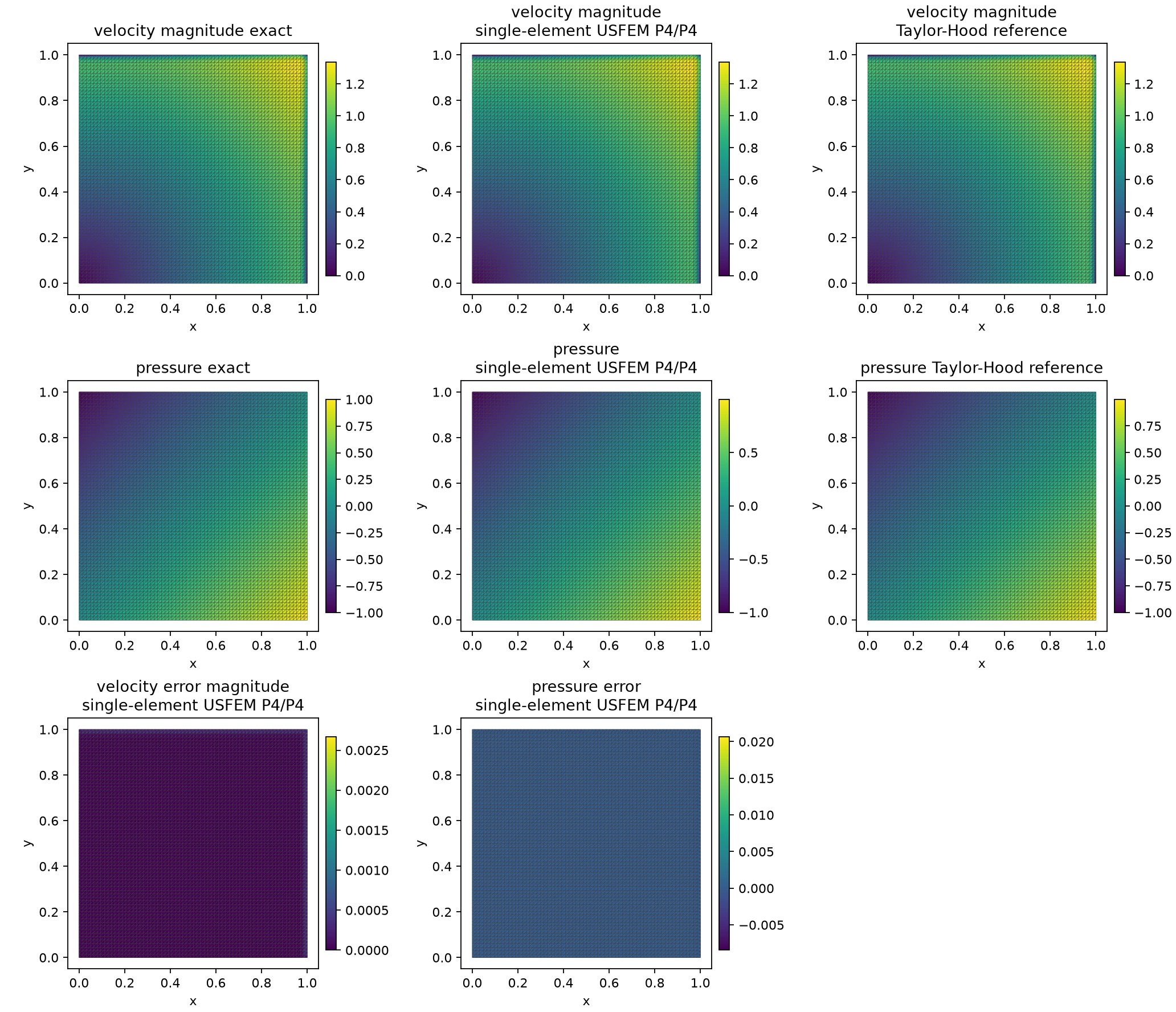
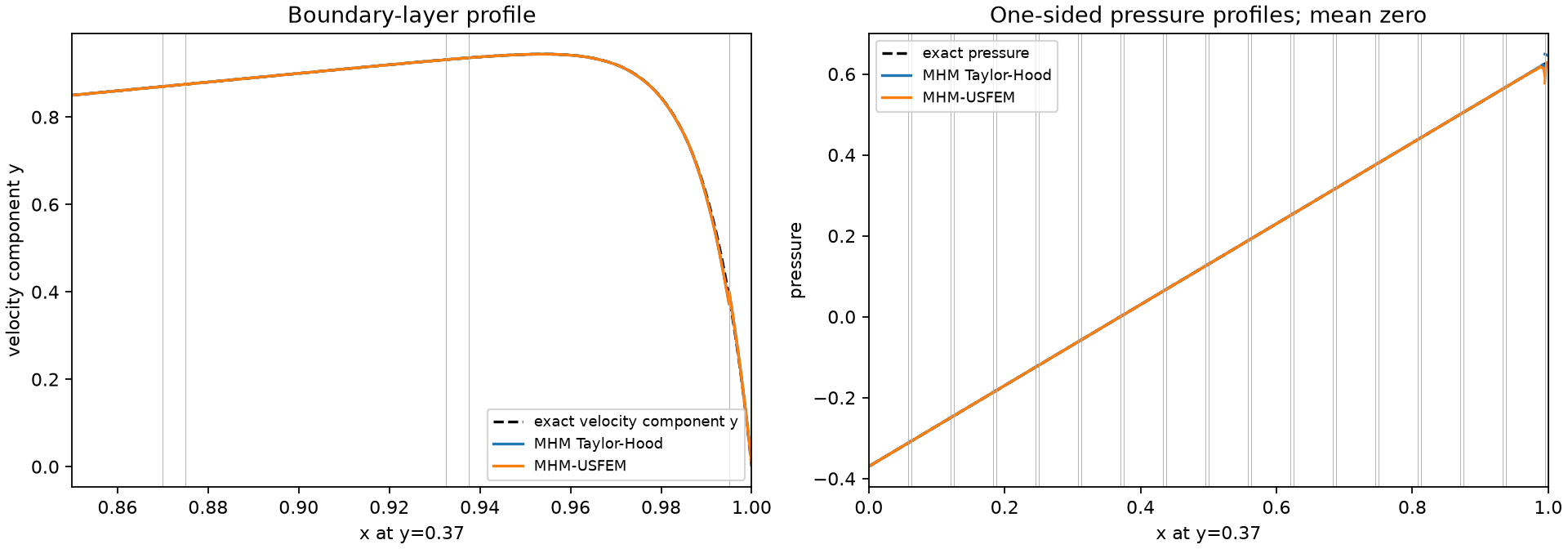
All analytical, numerical and error fields show the actual macro mesh; profile markers identify macroface crossings. Independently reconstructed incident values remain separate. The notebook measures velocity, pressure, velocity gradient, fine-cell divergence and macro mass balance. Macro conservation does not establish pointwise incompressibility or an H(div) velocity reconstruction.

7. Finish with asymptotic rates on smooth data

The difficult layer's measured P2/P2, P3/P3 and P4/P4 sequences are documented in the canonical boundary-layer case. They approach the reported orders as the layer resolves, with their pre-asymptotic slopes stated explicitly.

Both smooth studies below use the analytical fields

\[ \begin{aligned} \psi(x,y)&=128x^2(1-x)^2y^2(1-y)^2,\\ \boldsymbol u&=(\partial_y\psi,-\partial_x\psi),\\ p(x,y)&=150(x-\tfrac12)(y-\tfrac12),\\ \boldsymbol f&=-\Delta\boldsymbol u+\nabla p. \end{aligned} \]

They have viscosity one, zero resistance and homogeneous exterior velocity. The positive prefactor of \(\psi\) reverses the velocity in the polynomial example of Araya et al. (2017), Section 3.1.1, while retaining its pressure. These are analytical qualifications of the formulations, rather than reproductions of that paper's figure; these studies do not establish the same rates for an unresolved boundary layer.

Stabilized equal-order local problems

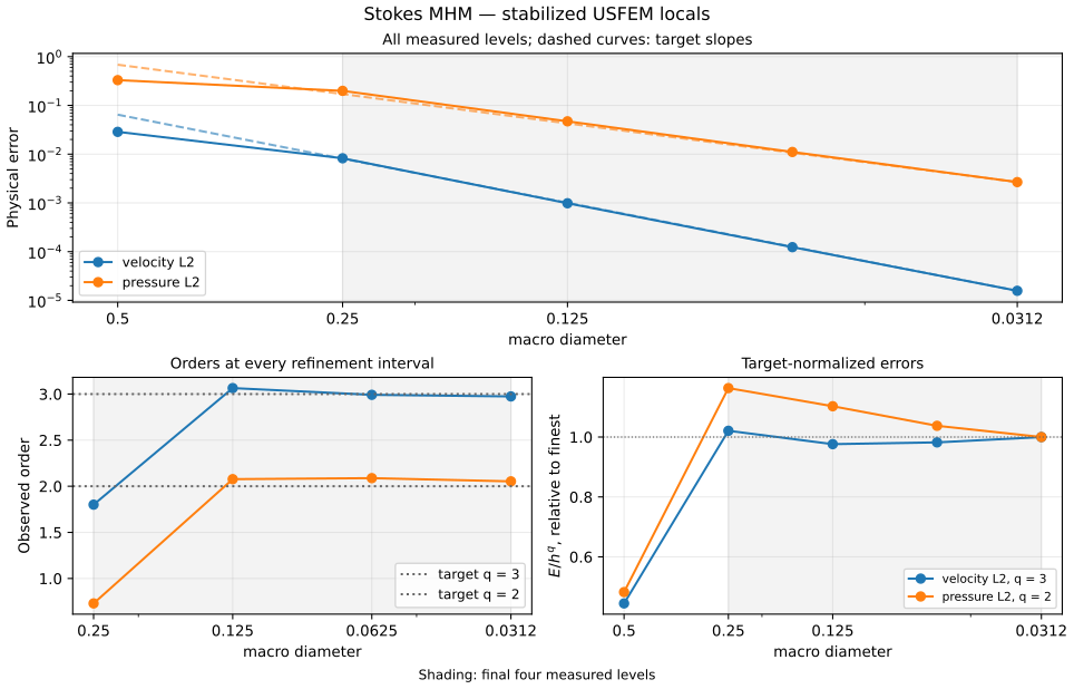
The stabilized family uses P3/P3 local fields and vector P1 traces on a crisscross macro mesh. Its pressure mean and translational local kernels are part of that source configuration. The smooth-data estimates require regular macroelements, admissible local lifting spaces, resolved local approximation and the stated pressure gauge. The final four levels are \(H=1/4,1/8,1/16,1/32\); the table shows all three intervals, rather than choosing only the final favorable slope. The normalized amplitude \(E/H^q\) is approximately constant in this window. Araya et al. (2017) and Araya et al. (2025) state the local stability, regularity and lifting hypotheses. The 2025 Theorem 4.2 estimates the broken velocity–pressure product norm, including the velocity gradient and pressure. The additional velocity \(L^2\) order three is observed in the 2017 experiments and the present smooth study; it is not a separate conclusion of that theorem.

Physical observable	Reference order	Last three orders	Maximum/minimum of \(E/H^q\)
velocity \(L^2\)	3	3.0644, 2.9914, 2.9741	1.0457
pressure \(L^2\)	2	2.0771, 2.0881, 2.0532	1.1635

Refined Taylor–Hood local Galerkin problems

The Galerkin variant has a separate refinement study. On each diagonal macrotriangle, divide each edge into four parts and use continuous P2 velocity and continuous P1 pressure on the resulting 16 fine triangles. The vector P1 multiplier remains unsplit on each macroface. In the pure Stokes problem, retain both velocity translations in the global formulation and impose the physical pressure integral once over the whole domain. These are the same kernel and gauge conventions used in the notebook's variational construction.

Section 2.2 of Araya et al. (2017) admits stable local Galerkin pairs, subject to the trace-lifting condition (48). The 2025 Theorem 4.3 gives a sufficient Taylor–Hood condition \(k-\ell\ge2\) in addition to Assumption (M). This P2/P1-local, P1-trace comparison has \(k-\ell=1\) and is outside that stated degree condition. Its concrete local operator and trace lifting are checked below; those checks do not establish the theorem for this broader family. The velocity \(L^2\) order three is additional measured accuracy.

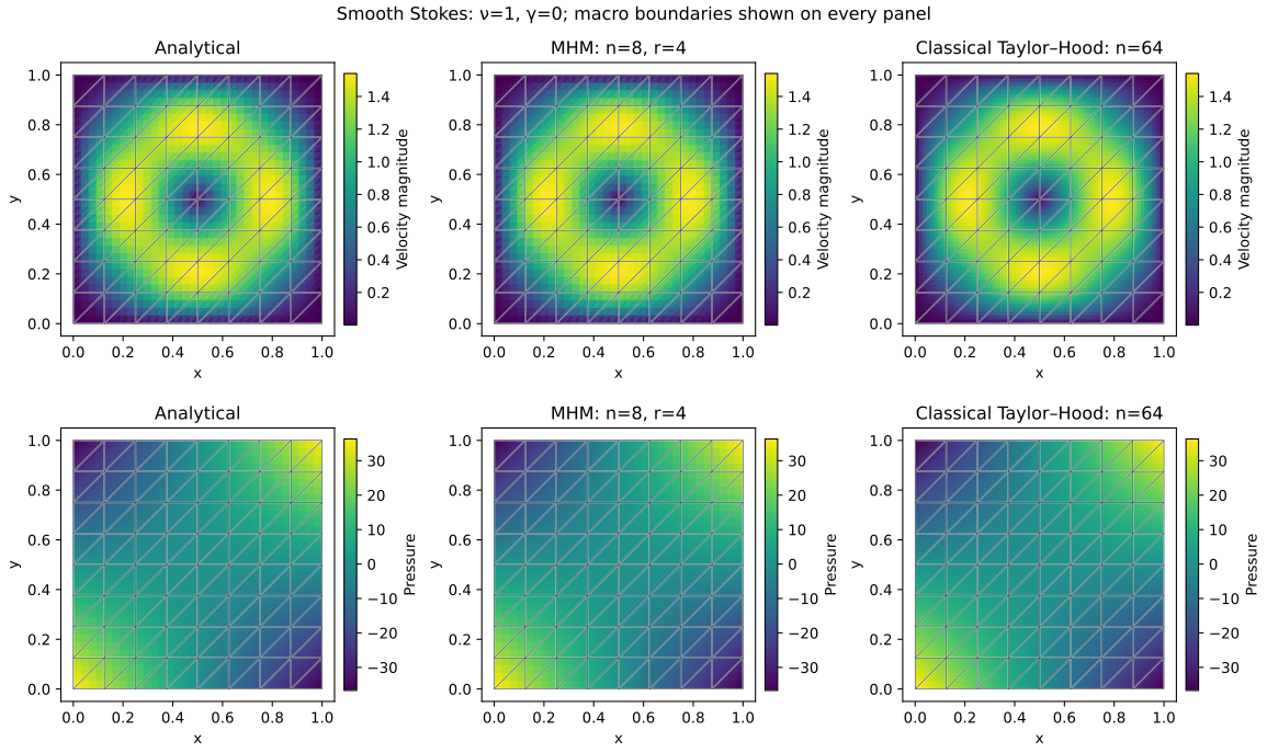
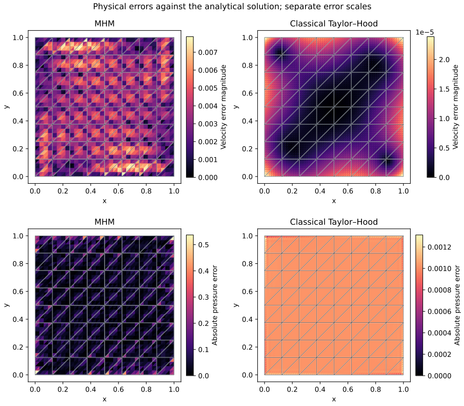
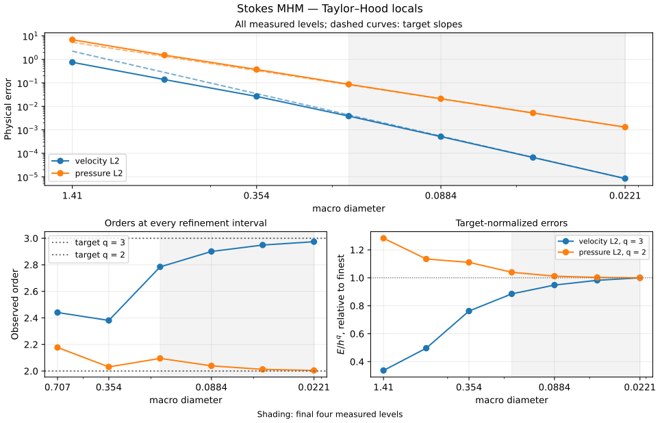
The illustration uses an \(8\times8\) macro grid with two diagonal triangles per square and a separate global Taylor–Hood reference on a \(64\times64\) grid. Every panel shows the actual macro mesh. The convergence study retains all seven macro-grid resolutions \(n=1,2,4,8,16,32,64\) and uses the actual triangle diameter \(H=\sqrt{2}/n\). Its final four levels give the following tail.

Physical observable	Observed reference order	Last three orders	Maximum/minimum of \(E/H^q\)
velocity \(L^2\)	3	2.9006, 2.9491, 2.9740	1.1300
pressure \(L^2\)	2	2.0392, 2.0125, 2.0043	1.0396

The independent UFL reference assembles the same Stokes operator and analytical source globally, with strong exterior velocity and zero physical pressure integral. Its own refinement is measured against the exact fields.

Global reference grid	Velocity \(L^2\) error	Pressure \(L^2\) error
\(32\times32\)	\(8.4796\times10^{-5}\)	\(9.4591\times10^{-3}\)
\(64\times64\)	\(1.0602\times10^{-5}\)	\(2.3640\times10^{-3}\)
\(128\times128\)	\(1.3255\times10^{-6}\)	\(5.9097\times10^{-4}\)

The local operator has exactly the two translational null modes in both triangle orientations. The divergence block has full pressure-row rank, and the P1 trace coupling has full rank on mean-free velocities. Independent UFL assembly also checks the volume operator, analytical source, signed trace coupling and physical moments. These finite-dimensional checks accompany the stability and regularity hypotheses; they are not uniform inf-sup estimates. The records check all original local momentum and incompressibility equations, global trace rows and the pressure gauge. Independent error quadratures of orders 12 and 16 agree on the measured norms.

References

• Rodolfo Araya, Christopher Harder, Abner H. Poza and Frédéric Valentin (2017). Multiscale hybrid-mixed method for the Stokes and Brinkman equations—The method. Computer Methods in Applied Mechanics and Engineering 324, 29–53. DOI: 10.1016/j.cma.2017.05.027.
• Rodolfo Araya, Christopher Harder, Abner H. Poza and Frédéric Valentin (2025). Multiscale Hybrid-Mixed Methods for the Stokes and Brinkman Equations—A Priori Analysis. SIAM Journal on Numerical Analysis 63(2), 588–618. DOI: 10.1137/24M1649368.