Parallel Darcy simulations

This application compares independent local solves on CPU workers and GPUs. It uses an oscillatory permeability and an analytical pressure so that the timed runs can also check pressure and the physical Darcy flux. The classical comparison solves the same operator with conforming Galerkin elements.

Problem and discretization

In two dimensions the domain is the unit square. The three-dimensional strong scaling cases use the unit cube; weak scaling extends it to \(\Omega_L=(0,L)\times(0,1)^2\) with integer \(L\). The data are

\[ \begin{aligned} p_*(\boldsymbol x)&=\prod_{j=1}^{d}\sin(\pi x_j),\\ K(\boldsymbol x)&=m_\varepsilon(\boldsymbol x)D,& m_\varepsilon(\boldsymbol x) &=\exp\!\left(\prod_{j=1}^{d}\sin(2\pi x_j/\varepsilon)\right),\\ \boldsymbol q&=-K\nabla p,& \nabla\cdot\boldsymbol q&=f=-\nabla\cdot(K\nabla p_*),\\ p&=0&&\text{on }\partial\Omega_L. \end{aligned} \]

Use \(D=I\) in 2D. The 3D permeability has the symmetric positive definite tensor

\[ D=\begin{pmatrix} 2&0.3&0.2\\ 0.3&1.5&0.1\\ 0.2&0.1&1 \end{pmatrix}. \]

The principal spatial period is \(\varepsilon=0.1\). A separate 3D experiment uses \(0.137\), which removes alignment between material oscillations and the macrofaces. Every macrocell assembles its own material matrix and prepares its own solver. Compiled forms and geometry-dependent workspaces can be shared.

For primal MHM, the local unknown \(p_T\) solves

\[ \begin{aligned} a_T(p_T,v)+b_T(v,\lambda)&=(f,v)_T,\\ a_T(p_T,v)&=\int_T K\nabla p_T\cdot\nabla v,\\ b_T(v,\lambda)&=\sum_{F\subset\partial T} s_{T,F}\int_F v\lambda_F. \end{aligned} \]

The global equations enforce the pressure pairing across macrofaces and retain the local constant compatibility rows. The signs \(s_{T,F}\) map the shared flux orientation to the outward normal of each macrocell. Local zero-mean responses and retained cell constants reconstruct the physical pressure.

The 2D default notebook uses \(200\times200\) fine quadrilaterals in total, local Q1 pressure and segmented P1 traces. The 3D CPU/GPU campaigns use 64 macrocubes per unit volume, local Q1 pressure and four tensor-Q1 trace coordinates on each unsplit macroface. A resolution \(n\) gives \(Ln^3\) fine hexahedra and \(n/4\) local subdivisions per direction.

Implementation

The notebooks declare the material, independently derived source, local UFL forms and global Equation before choosing an execution policy. For an already declared problem, change CPU execution without changing its forms:

from pymhm import ExecutionConfig, assemble, solve

execution = ExecutionConfig(backend="process", workers=8)
system = assemble(problem, execution=execution)
solution = solve(system)

Use backend="serial" for the serial comparison and backend="thread" for threads. Process providers are defined in importable modules, and process launches have a __main__ guard. The CPU guide, GPU guide and solver guide describe the individual settings.

The three complete implementations are available as rendered notebooks:

Measured scaling

Complete 3D process speedup with the ideal linear reference

CPU weak scaling at fixed local work per process

One- and two-GPU complete workflow measurements

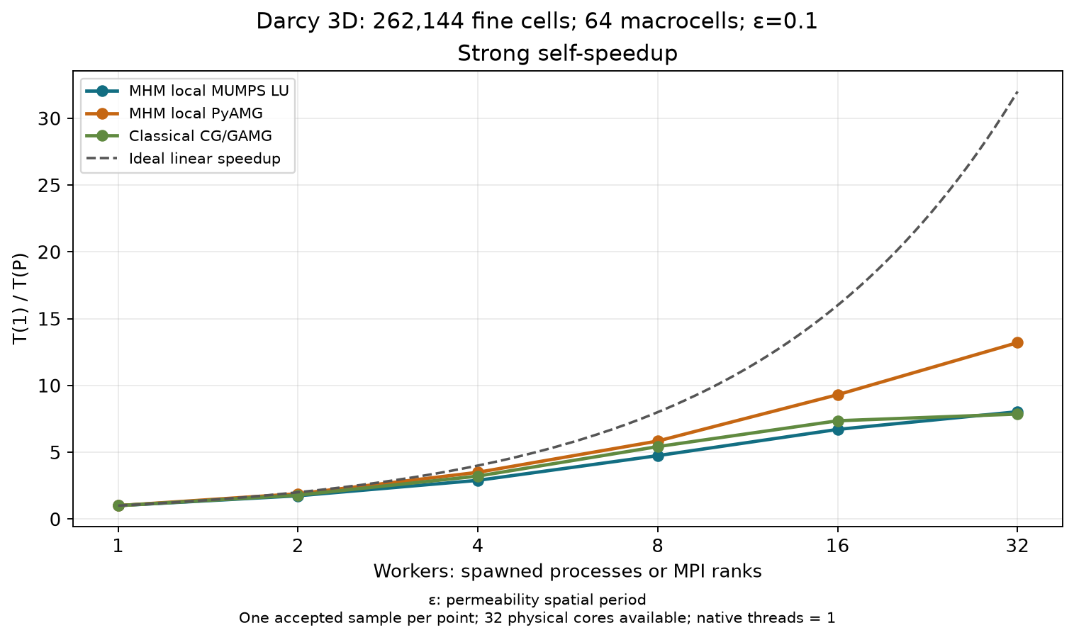
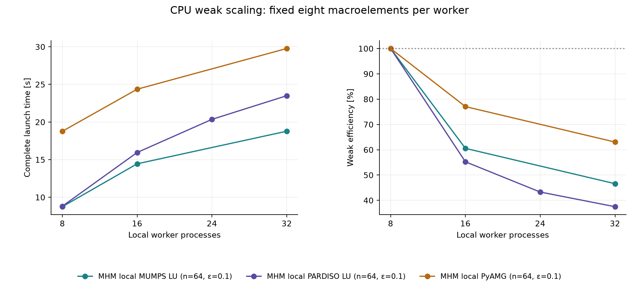
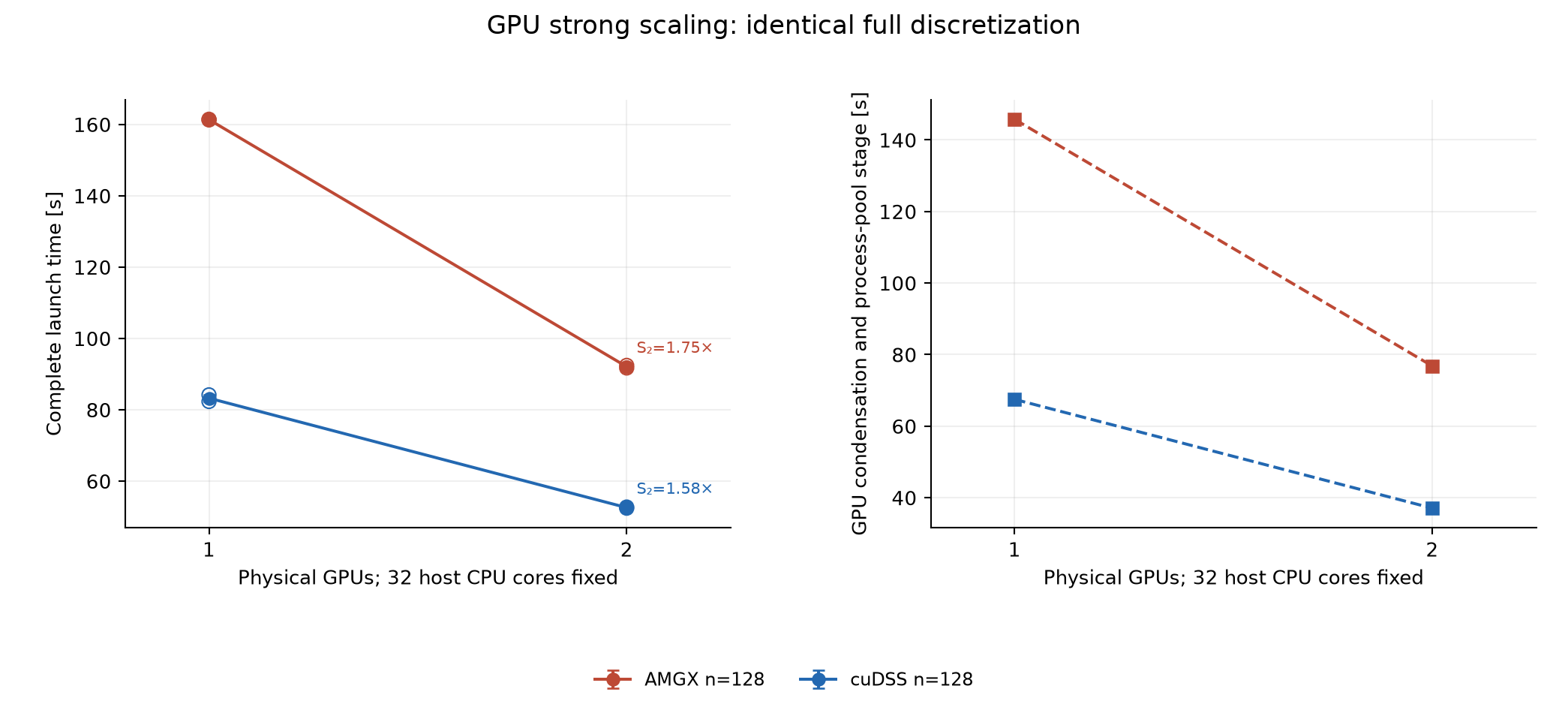
Strong scaling holds the physical discretization fixed; weak scaling grows the domain at fixed local work. Complete wall times include setup, communication, global assembly/solve and reconstruction. The reports distinguish them from the local-solver stage, and retain repetitions and the serial baseline.

The conforming and MHM approximation spaces differ even when they have the same total fine-element count. Their pressure and Darcy-flux errors are therefore shown alongside timings. The measured campaigns include configurations where parallel MHM is slower than a classical solve.

See the CPU workspace and LU/AMG report and CPU/GPU report for configuration tables, hardware, source identities and all measured clocks. Those plots retain their acquisition revisions; running the current notebooks produces new results for the current installation.

References

Christopher Harder, Diego Paredes and Frédéric Valentin (2013). A family of Multiscale Hybrid-Mixed finite element methods for the Darcy equation with rough coefficients. Journal of Computational Physics 245, 107–130. DOI: 10.1016/j.jcp.2013.03.019.
Antônio Tadeu A. Gomes, Weslley S. Pereira, Frédéric Valentin and Diego Paredes (2017). On the Implementation of a Scalable Simulator for Multiscale Hybrid-Mixed Methods. arXiv:1703.10435v1.