Incompressible Brinkman boundary layers

This analytical velocity/pressure problem contains exponential layers near the upper and right walls. MHM with Taylor–Hood local spaces and MHM-USFEM with equal-order local spaces solve the same physical operator, boundary data and pressure gauge.

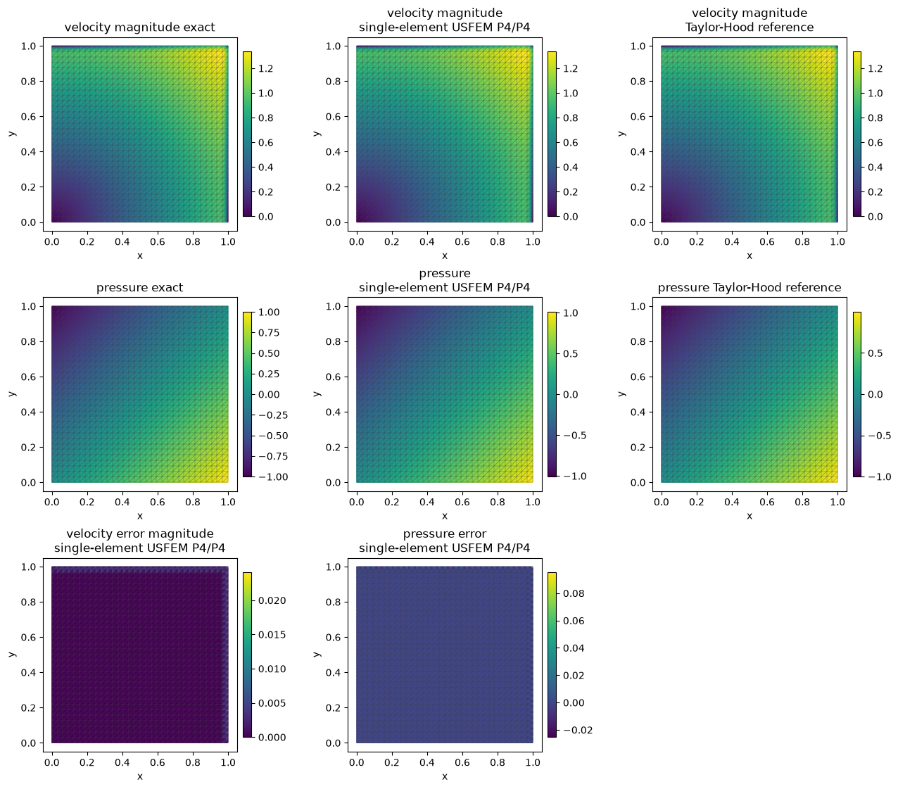
Physical problem

On \(\Omega=(0,1)^2\), the vector-Laplacian Brinkman equation is

\[ \begin{aligned} -\nu\Delta\boldsymbol u+\gamma\boldsymbol u+\nabla p&=\boldsymbol f, &\nabla\cdot\boldsymbol u&=0,\\ \nu&=10^{-2}, &\gamma&=1. \end{aligned} \]

The independently defined analytical fields are

\[ \begin{aligned} g(s)&=\frac{e^{(s-1)/\nu}-e^{-1/\nu}}{1-e^{-1/\nu}},\\ \boldsymbol u_*&=(y-g(y),\,x-g(x)), &p_*&=x-y,\\ \boldsymbol f&= \frac{(e^{(y-1)/\nu},e^{(x-1)/\nu})} {\nu(1-e^{-1/\nu})} +\gamma\boldsymbol u_*+(1,-1). \end{aligned} \]

Velocity equals \(\boldsymbol u_*\) on the complete exterior; pressure has zero volume mean. The layer width is \(\nu\) for these manufactured data.

Multiscale formulation and implementation

For each macrotriangle, the symmetric saddle form is

\[ \begin{aligned} a_T((\boldsymbol u,p),(\boldsymbol v,q)) &=(\nu\nabla\boldsymbol u,\nabla\boldsymbol v)_T +(\gamma\boldsymbol u,\boldsymbol v)_T\\ &\quad-(p,\nabla\cdot\boldsymbol v)_T -(q,\nabla\cdot\boldsymbol u)_T. \end{aligned} \]

The local interface variable is \(\boldsymbol\lambda_F=(-\nu\nabla\boldsymbol u+pI)\boldsymbol n_F\), the negative vector-Laplacian pseudotraction. The global equations enforce velocity-continuity moments, prescribed exterior velocity, and the single physical mean-pressure constraint. Symmetric Cauchy stress would define a different boundary form.

The local UFL form in the application mirrors the variational equation:

a = (
    nu * ufl.inner(ufl.grad(u), ufl.grad(v))
    + gamma * ufl.inner(u, v)
    - p * ufl.div(v)
    - q * ufl.div(u)
) * dx
load = ufl.inner(force, v) * dx

USFEM additionally subtracts the momentum-residual pairing \(\sum_\tau\tau_\tau(R(\boldsymbol u,p),R(\boldsymbol v,q))_\tau\) and its matching source term, where \(R=-\nu\Delta\boldsymbol u+\gamma\boldsymbol u+\nabla p\). The inverse bound is evaluated on the executed local polynomial space.

The complete application defines these residuals, spaces, boundary coupling and gauge before assembly. Four local subdivisions supply interior vertices for the 2D Taylor–Hood \(P_2/P_1\) submesh. Its equal-order USFEM comparison uses the same local velocity mesh and trace space. Separate single-element \(P_{\ell+2}/P_{\ell+2}\) families use the literature's unsplit traces.

Results and reproducibility

Velocity, pressure, gradient and divergence are evaluated separately against the exact fields. A classical conforming Taylor–Hood reference is also refined independently on the same data. Macro mass balance and fine-cell divergence are distinct diagnostics.

The unsplit-trace single-element family with \(\ell=2\) and 64 macro divisions has velocity L2 error \(6.0896\times10^{-5}\), pressure L2 error \(2.4764\times10^{-4}\) and gradient error \(3.569\times10^{-2}\). These recorded layer results are distinct from the smooth asymptotic qualification in the Stokes–Brinkman tutorial.

The application notebook and downloads include analytical fields, one-sided profiles, error integration and precise space/parameter records. The result report retains measured refinement slopes and independently assembled checks. Historical mesh connectivity and inverse constants are not completely specified by the article; agreement with every original plotted ordinate is not asserted.

References

• Rodolfo Araya, Christopher Harder, Abner H. Poza and Frédéric Valentin (2017). Multiscale hybrid-mixed method for the Stokes and Brinkman equations—The method. DOI: 10.1016/j.cma.2017.05.027.
• Rodolfo Araya, Christopher Harder, Abner H. Poza and Frédéric Valentin (2025). Multiscale Hybrid-Mixed Methods for the Stokes and Brinkman Equations—A Priori Analysis. DOI: 10.1137/24M1649368.