Extension of a heterogeneous solid

A plane-strain solid undergoes a one-percent horizontal extension. Short material wavelengths generate nonuniform strains inside each macroelement. The comparison shows how local resolution improves stress prediction while keeping a small global system.

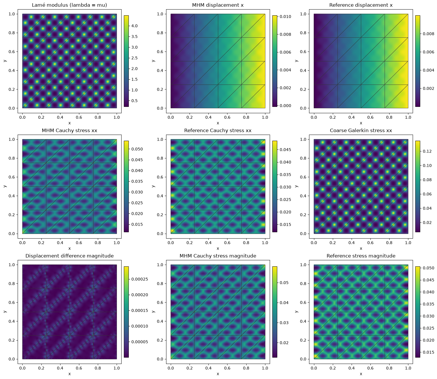
The upper-left panel shows the prescribed material coefficient \(\lambda=\mu\). The other panels show computed displacement, Cauchy stress and the displacement difference from the refined numerical reference. Every panel overlays the actual macro mesh.

Physical problem

On \(\Omega=(0,1)^2\), there is no body force and displacement is prescribed on the whole exterior:

\[ \begin{aligned} -\nabla\cdot\boldsymbol\sigma&=0, &\boldsymbol u_D&=(0.01x,0),\\ \boldsymbol\sigma&=2\mu\varepsilon(\boldsymbol u) +\lambda\nabla\cdot\boldsymbol u\,I,\\ \varepsilon(\boldsymbol u)&=\tfrac12 \left(\nabla\boldsymbol u+\nabla\boldsymbol u^{\mathsf T}\right),\\ \lambda(x,y)=\mu(x,y)&= \exp\left(1.5\sin(16\pi x)\sin(16\pi y)\right). \end{aligned} \]

The material wavelength is \(1/8\) and its contrast is \(e^3\simeq20.1\). The plane-strain Poisson ratio is \(1/4\): this application isolates heterogeneity rather than near-incompressibility.

Multiscale formulation and implementation

Primal MHM uses local vector-valued \(P_3\) displacement and a globally oriented negative Cauchy traction. Each local problem has the strain-energy form

\[ a_T(\boldsymbol u,\boldsymbol v)= \int_T2\mu\varepsilon(\boldsymbol u):\varepsilon(\boldsymbol v) +\lambda(\nabla\cdot\boldsymbol u)(\nabla\cdot\boldsymbol v). \]

The local equation adds \(\langle s_{TF}\boldsymbol\lambda,\boldsymbol v\rangle_{\partial T}\). The global equation enforces displacement-jump moments and the prescribed exterior displacement. Two translations and one rotation are retained per macrotriangle; the local energy complement is fixed by their physical moments. The exterior data remove global rigid-motion ambiguity.

The provider expresses these terms directly in UFL:

a = (
    2 * mu * ufl.inner(ufl.sym(ufl.grad(u)), ufl.sym(ufl.grad(v)))
    + lam * ufl.div(u) * ufl.div(v)
) * dx
b = local.trace_pairings(lambda phi, ds: ufl.inner(phi, v) * ds)
c = local.trace_pairings(lambda phi, ds: -ufl.inner(phi, u) * ds, axis="rows")
local.field("displacement", binding)

The rendered application defines the local space, rigid modes and moments, global equation, solver, physical Cauchy stress and comparisons. The primal elasticity tutorial explains this method on an analytical problem.

Results and reproducibility

The MHM global system has 992 unknowns, with at most 2,450 local unknowns. An independently assembled conforming \(P_2\) baseline is refined over \(64\times64\), \(128\times128\) and \(256\times256\) square grids split into triangles. The finest reference has 526,338 displacement unknowns.

Relative differences from the finest reference are 0.482% in displacement L2 and 13.78% in Cauchy-stress L2 for MHM. A classical solve on the coarse macro mesh gives 1.927% and 99.35%, respectively. The last reference refinement changes stress by 1.165%; it measures reference sensitivity, rather than a certified remaining error. There is no analytical solution for this material/loading pair.

The application notebook and downloads declare the displacement coordinate basis, integration controls and original-equation checks. Both local and conforming forms solve the same material and boundary problem; the reference assembly shares the native DOLFINx/Basix backend.

References

• Christopher Harder, Alexandre L. Madureira and Frédéric Valentin (2016). A hybrid-mixed method for elasticity. DOI: 10.1051/m2an/2015046.