Reaction–diffusion boundary layers
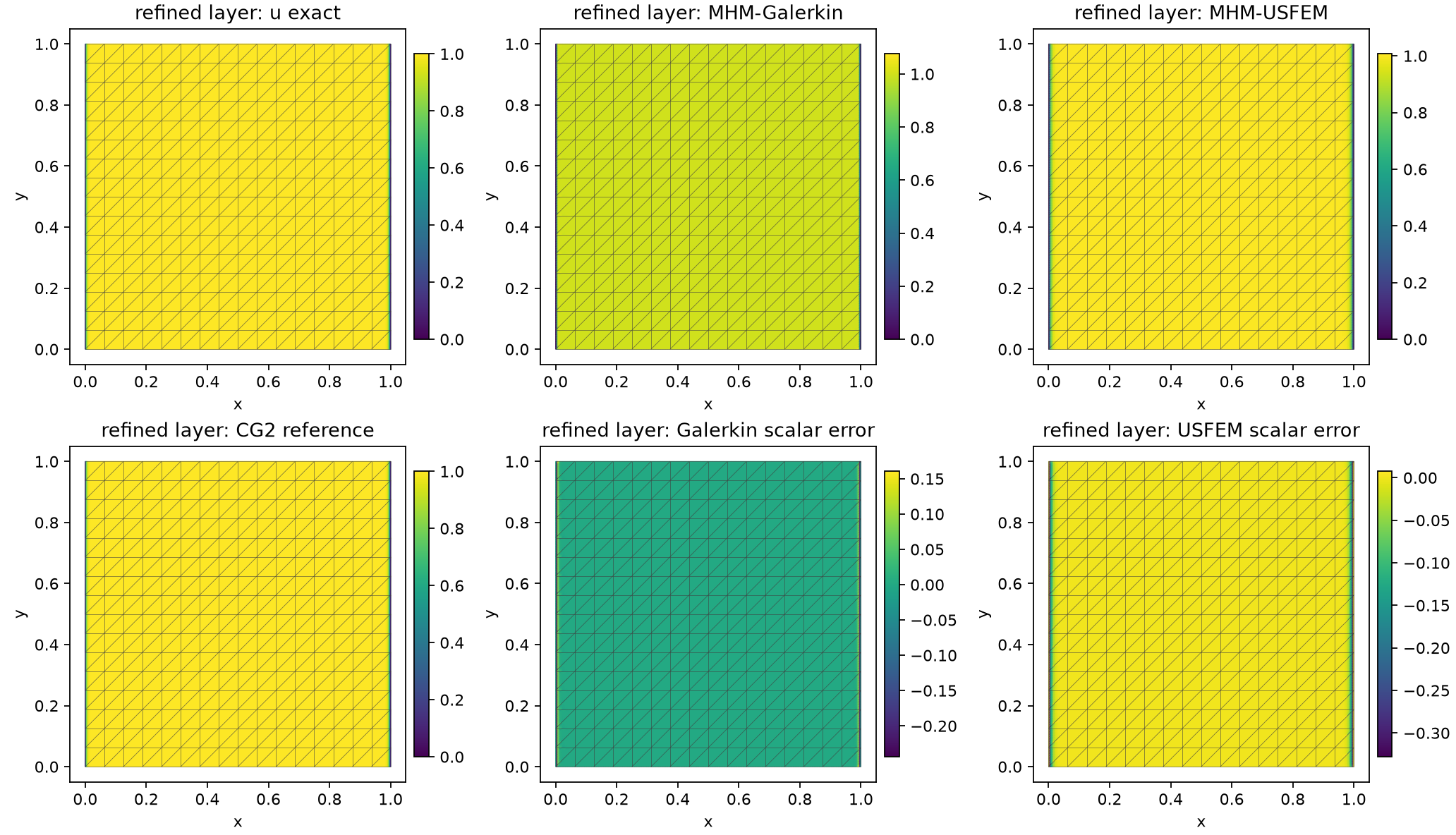
Small diffusion creates two thin boundary layers that coarse local finite elements cannot resolve. This application compares ordinary Galerkin and MHM-USFEM local solves on the same macro mesh, separating suppression of overshoots from accuracy of the physical fields.
Physical problem
On the unit square, diffusion is constant, reaction and source equal one:
The independent exact solution is
The layer width is of order \(\sqrt\epsilon\): approximately 0.0316 for \(\epsilon=10^{-3}\) and 0.00316 for \(\epsilon=10^{-5}\).
Multiscale formulation and implementation
Local fields use continuous \(P_1\) on affine fine triangles; each macroface has four independent \(P_0\) segments in the resolved family. Eight local subdivisions per macroedge provide the additional red refinement required by this trace/local pairing.
With \(Lw=w-\epsilon\Delta w\), the USFEM local equation uses
Ordinary Galerkin omits both residual terms. In both methods, the local equation adds the oriented diffusive-flux pairing; the global equation imposes scalar-continuity moments on interior faces. Vertical Dirichlet values are imposed strongly, and horizontal normal-flux coordinates are zero. Positive reaction removes the constant local kernel.
The local volume forms are declared directly:
def strong(w):
    return w - epsilon * ufl.div(ufl.grad(w))


a = (epsilon * ufl.inner(ufl.grad(u), ufl.grad(v)) + u * v) * dx
load = v * dx
if stabilized:
    a -= tau * strong(u) * strong(v) * dx
    load -= tau * strong(v) * dx
The MHM-USFEM tutorial provides the complete local/global declarations and runnable notebook. The boundary-layer result report specifies both coarse and refined configurations and reference meshes.
Results
At \(\epsilon=10^{-5}\) and 16 macro divisions, Galerkin and USFEM scalar L2 errors are 0.02018 and 0.03312. Their nodal overshoots are 0.07594 and 0.00688: stabilization markedly reduces the overshoot while broadening the unresolved layer. Its scalar error is larger in this configuration.
Physical-flux L2 errors are \(1.0181\times10^{-4}\) and \(1.0318\times10^{-4}\), approximately 57.3% and 58.0% of the exact flux norm. This severe-layer sequence remains underresolved. The comparison retains that limitation; smoother analytical rate studies in the method tutorial answer a different question.
The independently assembled conforming CG2 reference uses up to \(1024\times16\) intervals and the same mixed boundary data. Its exact scalar and flux errors are \(2.4000\times10^{-5}\) and \(6.0713\times10^{-7}\). Every spatial plot marks the actual macro mesh; profiles preserve the independent values on each side of a macroface.
References
- Larissa Martins, Juan F. Pacazuca and Frédéric Valentin (2025). A Multiscale Hybrid-Mixed Method with Local Stabilization. CILAMCE proceedings, DOI: 10.55592/cilamce2025.v5i.14270.