Independent NeoPZ comparison
An independent mixed finite element assembly can check the local Darcy operators, face orientations, pressure reconstruction, and MHM condensation against another implementation. This comparison uses NeoPZ's public RT0 element family on exactly the same triangular mesh. It also distinguishes that reference from Labmec's higher-order mixed MHM controller.
An additional coarse cosine check uses the gallery's exact 32-macrotriangle, 512-fine-triangle configuration. It reproduces its 21.8662% flux error and compares the complete RT0 fields.
The reference uses NeoPZ commit
4c6b6d2
and Labmec/MHM commit
f978f29.
Execution with the independent driver tests the same discrete equations; it
does not constitute execution of an unchanged historical MHM application.
Spaces that can be compared exactly
The native mixed Darcy solver uses
There is one flux integral per oriented fine edge and one pressure value per fine triangle. The divergence belongs to \(P_0(T)\). The skeleton represents the physical normal flux, with a fixed normal for each macroedge.
NeoPZ's public EHDivConstant family constructs RT0 facet modes and enriches
them by divergence-free curls. At order zero, no enrichment modes remain:
there are three flux DOFs on a triangle, and the basis is RT0. The name
"constant" describes its divergence; an RT0 vector field can vary linearly
inside an element. See the basis construction and
DOF count. This order-zero family is used by the independent
reference.
The positive-order EHDivStandard family used by the mixed MHM controller is
different. Its triangular flux count is
For example, standard order one has nine flux DOFs, rather than the eight of classical RT1. The disconnected pressure space has degree \(k\), while the normal trace has degree \(k\). The controller can additionally raise the interior flux and pressure degrees without raising the skeletal degree. Matching the integer degree alone therefore does not establish matching spaces. See standard DOF counts, pressure construction, and interior enrichment.
The mixed MHM controller requires positive interior and skeleton degrees;
its skeleton-order setter maps nonpositive values to one. The RT0 reference
instead uses the order-zero EHDivConstant family. These are distinct
approximation spaces and execution paths. See the
controller degree requirements.
The historical application's default mesh uses quadrilaterals and its default interior/skeleton degrees are two/one. Replacing those elements by triangular RT0 changes the approximation. The independent RT0 comparison is valuable because its spaces agree with the native solver, but it must not be labelled a reproduction of that default application. The application configuration and mesh generator make this distinction explicit.
Matching signs, orientations, and pressure
NeoPZ's mixed material and pyMHM use the same weak equations:
Dirichlet pressure is imposed through boundary moments. The modern NeoPZ material used by the independent driver supports scalar isotropic permeability; comparisons therefore use \(K=kI\). The volume contributions and boundary contributions provide the reference signs.
For a counterclockwise triangle with area \(|T|\), pyMHM writes the RT0 basis associated with an edge opposite vertex \(\boldsymbol a_e\) as
Here \(s_{Te}\) compares the cell's outward normal with the globally chosen normal. NeoPZ implements the contravariant Piola map and carries orientation through its side signs and permutations. These are equivalent on the affine triangles of this comparison. Raw basis coefficients need not share signs or normalization; compare physical flux samples and integrals against a common normal. See NeoPZ's Piola map.
pyMHM's constrained local pressure lift has zero volume mean, and its coarse pressure amplitude restores a constant. NeoPZ's mixed controller instead keeps an algebraic pressure connect before condensation. That retained coefficient is not generally the physical macrocell mean. Compare reconstructed pressure and integrated means, not coarse coefficient vectors. See the retained-connect algorithm.
For pure Neumann conditions a common global pressure gauge is also necessary. Keeping a local pressure connect does not remove the global additive constant. The NeoPZ material imposes Neumann flux by a large penalty, whereas pyMHM fixes projected flux coefficients strongly. The recorded comparison uses Dirichlet conditions. An equivalent Neumann comparison requires matching flux imposition and the pressure gauge.
Full and restricted skeletal traces
When each macroedge has one P0 skeleton segment per fine edge, the skeleton spans every admissible RT0 normal trace. MHM condensation must then recover the global conforming RT0/P0 solution on the assembled fine mesh. This tests the local operators and elimination against an independent global assembly.
For a genuinely restricted MHM space, let \(T\) map a vector of independent coarse flux and pressure coordinates to the full mixed reference coordinates. The restriction affects interface fluxes; fine interior fluxes and fine pressure values remain independent before condensation. If the global mixed reference system is \(A x=b\), the restricted equations are
Flux entries of \(T\) must account for face orientation and physical lengths. For a constant macroedge flux, a fine-edge integral equals that flux times the fine-edge length with the corresponding sign. Restricting just coefficient indices without those factors can change the problem. Comparing this system with pyMHM's reduced trace tests MHM approximation as well as condensation. It is a restricted-trace NeoPZ reference, separate from the positive-order historical controller. That controller applies its own facet dependencies.
Comparison results
The executed study contains 46 comparisons: 23 with the complete fine-edge trace and 23 with a constant trace on each macroedge. The Cartesian macro grid has \(n=1,2,4,8,16\) squares per axis, split into triangles; each macrotriangle is subdivided with \(r=2\). Thus there are \(2n^2\) macrotriangles and \(8n^2\) fine triangles. The two layered cases use \(n=2,4,8,16\) so that the material interface coincides with mesh edges. All cases impose exact pressure on the exterior boundary and use the same geometry in both implementations.
| Case | Exact pressure \(p\) | Permeability | Source \(f\) |
|---|---|---|---|
| Affine | \(1+x+2y\) | \(K=I\) | \(0\) |
| Polynomial | \(x^2+y^2+xy\) | \(K=I\) | \(-4\) |
| Cosine | \(\cos(\pi x)\cos(\pi y)\) | \(K=I\) | \(2\pi^2p\) |
| Layered | \(1+\min(x,\tfrac12)+\max(x-\tfrac12,0)/10+2y\) | \(K=kI\), \(k=1\) left and \(10\) right | \(0\) |
| Layered, contrast \(10^3\) | \(1+\min(x,\tfrac12)+\max(x-\tfrac12,0)/1000+2y\) | \(K=kI\), \(k=1\) left and \(1000\) right | \(0\) |
The layered solutions have \(\boldsymbol q=(-1,-2k)\): normal flux is continuous across \(x=1/2\), while the tangential component jumps. Their exact flux belongs to both discrete spaces; their nonconstant pressure cannot be represented exactly by P0. An affine pressure likewise has a nonzero P0 approximation error even when its constant flux is recovered to roundoff.
The RT0 Dirichlet functional depends only on the pressure average on each fine boundary edge. The reference supplies that average, computed by NeoPZ's Gauss rule requested at order 20 (11 points), as a constant boundary value. This represents the same discrete Dirichlet functional. Divergence is evaluated from the native H(div) divergence solution field; see H(div) solution evaluation.
The reference with two trace segments per macroedge (\(s=2\)) uses the native NeoPZ skyline LDLt solve. The reference with one segment (\(s=1\)) uses the independently assembled NeoPZ matrix, the restriction described above, and a SciPy sparse solve; its coefficient vector is then imported into NeoPZ for native field evaluation. Neither reference uses pyMHM's assembled matrices.
The table gives the largest absolute field differences in L2 across the listed meshes. Differences of RT0 fields are integrated exactly with a three-point, degree-two triangle rule. Error norms against the analytical solution use a separate Duffy order-10 rule. These are comparisons of physical fields, not just comparisons of their error norms.
| Case | Segments \(s\) | Meshes | \(\lVert p_{\rm pyMHM}-p_{\rm ref}\rVert\) | \(\lVert \boldsymbol q_{\rm pyMHM}-\boldsymbol q_{\rm ref}\rVert\) | \(\lVert \nabla\cdot(\boldsymbol q_{\rm pyMHM}-\boldsymbol q_{\rm ref})\rVert\) |
|---|---|---|---|---|---|
| Affine | 2 | 5 | 3.84e-13 | 1.82e-12 | 3.40e-11 |
| Polynomial | 2 | 5 | 1.34e-13 | 6.72e-13 | 1.63e-11 |
| Cosine | 2 | 5 | 1.39e-11 | 7.12e-11 | 5.67e-12 |
| Layered, contrast 10 | 2 | 4 | 1.53e-13 | 7.88e-12 | 2.87e-10 |
| Layered, contrast 1000 | 2 | 4 | 1.04e-13 | 3.93e-10 | 2.25e-8 |
| Affine | 1 | 5 | 2.83e-15 | 5.07e-14 | 3.10e-13 |
| Polynomial | 1 | 5 | 9.04e-16 | 2.05e-14 | 1.22e-13 |
| Cosine | 1 | 5 | 1.57e-11 | 7.12e-11 | 3.26e-13 |
| Layered, contrast 10 | 1 | 4 | 2.12e-15 | 3.00e-13 | 2.75e-13 |
| Layered, contrast 1000 | 1 | 4 | 3.50e-14 | 9.04e-11 | 1.39e-11 |
Pressure and flux acceptance thresholds are \(10^{-9}\max(1,\|u_{\rm ref}\|)\) for the respective field. The divergence threshold is \(10^{-8}\max(1,\|\boldsymbol q_{\rm ref}\|,\|\nabla\cdot\boldsymbol q_{\rm ref}\|)\). All 46 cases pass these fixed checks. In the contrast-1000 case the flux norm is approximately \(1.414\times10^3\), so the largest flux difference corresponds to about \(2.8\times10^{-13}\) relative to that norm.
Conservation is checked by integrating \(\nabla\cdot\boldsymbol q_h-f\) in each fine cell using the assembly source quadrature. The maximum absolute integrated defect is \(1.14\times10^{-13}\) in pyMHM and \(8.42\times10^{-11}\) in the reference, over all 46 cases. For the full-trace contrast-1000 case, the larger divergence-density difference in the table accompanies a much smaller integrated defect: differentiating fine-cell fields amplifies flux coefficient errors. Both measures remain recorded, rather than using the integrated residual alone to assess agreement.
Boundary quadrature sensitivity
The recorded cosine comparisons use five Gauss points per skeleton segment for pyMHM boundary moments and 11 Gauss points for the NeoPZ boundary means. A controlled integration study compares the five-point rule with a 20-point rule for pyMHM's boundary moments, keeping the volume quadrature, finite element spaces, reference fields and solver tolerances fixed.
| Configuration | Flux difference, 5 points | Flux difference, 20 points |
|---|---|---|
| \(n=1\), \(s=2\) | 7.1241e-11 | 5.1509e-14 |
| \(n=2\), \(s=1\) | 7.1241e-11 | 1.7045e-15 |
The reduction in field differences identifies boundary integration as the leading discrepancy in these two coarse cosine cases. The 46 comparisons reported above use the five-point pyMHM rule and the 11-point NeoPZ rule.
Convergence and physical fields
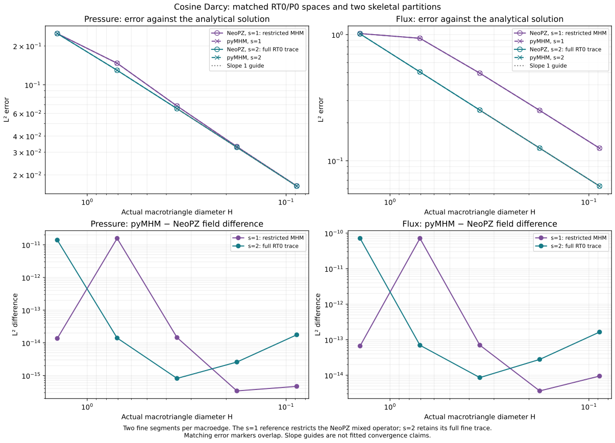
The expected asymptotic rate is first order for RT0 flux and P0 pressure. With \(r=2\) fixed, reducing the macrotriangle diameter \(H=\sqrt{2}/n\) refines both macro and fine meshes. The five measured levels approach that rate. A single constant trace per macroedge has a larger flux error than the complete trace, as expected from the smaller approximation space. Its coarsest two flux errors are almost stationary; both points are retained. The reference and pyMHM convergence curves overlap to the field differences reported above.
For example, at \(n=16\) the pressure/flux errors are \(0.0163597/0.0629614\) with \(s=2\) and \(0.0164147/0.125766\) with \(s=1\). Near-zero errors in the representable affine and layered fluxes are consistency checks, not convergence-rate measurements.
The figure reads the retained pressure/flux errors and field differences against the declared macrogeometry; its rendering provenance records the original report digest and all five diameters. It does not reconstruct spatial fields from scalar errors. The original 46 coefficient archives are not distributed, so spatial panels and one-sided profiles for those acquisition files cannot be replayed from this checkout.
The separate coarse cosine field comparison includes downloadable P0/RT0 field data, native NeoPZ reevaluation and actual macro boundaries. Its configuration is \(n=4\), \(r=4\), \(s=1\), rather than the \(r=2\) refinement series above. Both methods share a substantial coarse-trace flux error even when their reconstructed fields agree to roundoff.
Restricted macro trace
The independent restriction retains all fine pressure and interior flux coordinates before condensation. The following dimensions therefore describe the reference systems, not pyMHM's condensed global system.
| \(n\) | Macrotriangles | Fine triangles | Full \(A\) | Restricted \(T^{\mathsf T}AT\), \(s=1\) |
|---|---|---|---|---|
| 1 | 2 | 8 | 24 | 19 |
| 2 | 8 | 32 | 88 | 72 |
| 4 | 32 | 128 | 336 | 280 |
| 8 | 128 | 512 | 1312 | 1104 |
| 16 | 512 | 2048 | 5184 | 4384 |
The maximum relative algebraic residual is \(1.78\times10^{-11}\) for the native full solves and \(2.30\times10^{-13}\) for the restricted solves. The latter check uses \(T^{\mathsf T}(ATy-b)\): the full unrestricted residual need not vanish for a constrained approximation. Native NeoPZ evaluation of the imported restricted coefficients gives the \(s=1\) field comparisons above.
Inspect the archived comparison
The executed C++ comparison driver is named neopz_rt0. It uses NeoPZ
for finite element assembly and field evaluation. The checkout provides complete
JSON measurements, field hashes and boundary-quadrature diagnostics. The original
46 coefficient archives and instrumented external driver are not distributed.
The standalone notebook assembles fresh RT0/P0 equations through the public API
for the same five analytical physical cases and reports pressure, physical-flux
and fine-cell equilibrium errors:
Results are in examples/results/neopz/comparison.json; the boundary diagnostic
is in examples/results/neopz/boundary-quadrature.json. Execution provenance
records source and archive SHA-256 digests. The accompanying
notebook reads the retained original provenance separately from
its current analytical refinement. Selecting --historical additionally loads
all 46 original coefficient archives, validates their recorded hashes and
displays their comparison figures. This option requires the original payloads;
newly solved fields do not recreate their acquisition identity. The
recorded execution establishes agreement for the tested
triangular RT0/P0 problems and trace restrictions. Higher-order spaces,
three-dimensional elements, Neumann penalties and unchanged historical MHM
drivers require separate comparisons.
RT0 trace compatibility
An RT0 normal trace is constant on each fine edge. The skeletal space must therefore consist of degree-zero segments whose endpoints coincide with fine boundary vertices. Each segment can span one or more complete fine edges; a segment boundary inside a fine edge is inadmissible.
With this compatibility condition, the reconstructed mixed field satisfies \(\boldsymbol q_h\cdot\boldsymbol n=\lambda_h\) on every fine boundary edge, using the common macroface normal. Matching only the integrated flux across a macroface is a weaker condition and does not establish this trace identity. The RT0 local-equation definition validates the polynomial degree and partition alignment before assembly; see the mixed MHM tutorial.