Transient transport MHM

Write the capacity-weighted mass, conservative transport and interface forms with UFL. A backward-Euler time loop updates physical source loads and previous concentration while the generic offline system reuses unchanged local and global operators.

Complete executable notebook · Download notebook

Run in introduction. The notebook declares the entire problem and time loop; it does not call a ready-made transport simulation. Two complementary notebooks separate temporal integration from spatial multiscale approximation. Spatial refinement notebook uses the same by-hand UFL local/global workflow with linear-time manufactured data.

1. Choose the physical concentration and initial data

On the unit square, capacity and diffusion are one, reaction is \(1/2\), and constant transport velocity is \(\beta=(1/4,-1/2)\):

\[ \begin{aligned} &\partial_t c+\nabla\cdot(-\nabla c+\beta c)+\tfrac12c=f,\\ c_*(x,y,t)&=e^{-t}\phi(x,y),\\ \phi(x,y)&=\sin(\pi x)\sin(\pi y),\\ f(x,y,t)&=e^{-t}\big[(2\pi^2-\tfrac12)\phi+\beta\cdot\nabla\phi\big]. \end{aligned} \]

The concentration is zero on the exterior. The source is derived from the PDE, not from the discrete matrix. Initial concentration is the independent physical \(L^2\) projection of \(\phi\). Physical transport flux and skeletal multiplier are

\[ j=-\nabla c+\beta c, \qquad\lambda_K=(-\nabla c+\tfrac12\beta c)\cdot n_K. \]

Their advection contributions differ. The multiplier is not the complete transport flux used in a physical conservation diagnostic. Harder et al. (2015) and Araya et al. (2024) give the underlying conservative hybrid formulation.

2. Bind macro, local and interface meshes

The spatial approximation remains unchanged through the time-refinement study: P2 concentration on fine triangles and segmented P1 normal traces. The local mesh has twice as many edge subdivisions as the interface partition, providing an enriched local trace lifting.

macro = TriangleMesh.unit_square(2)
local_refinement = 16
skeleton = SkeletonSpace(
    macro,
    tuple(FaceSpace.uniform(1, local_refinement//2) for _ in macro.faces),
)
hierarchy = MeshHierarchy(
    macro, tuple(macro.submesh(i, local_refinement) for i in range(len(macro.cells))),
)
interface = bind_interface(skeleton, convention="normal")

The binding supplies incident orientation and geometric support. A trace space richer than the independent local boundary responses can introduce redundant multipliers; it is not repaired by a solver perturbation.

3. Translate backward Euler into a local equation

For a step of length \(\Delta t\), the local equation is

\[ \begin{aligned} \tfrac1{\Delta t}(c_K^{n+1},v)_K+a_K(c_K^{n+1},v) +\langle\lambda_K^{n+1},v\rangle_{\partial K} &=(f^{n+1},v)_K+\tfrac1{\Delta t}(c_K^n,v)_K,\\ a_K(c,v)&=(\nabla c,\nabla v)_K+\tfrac12(c,v)_K\\ &\quad+\tfrac12[(\beta\cdot\nabla c,v)_K-(c,\beta\cdot\nabla v)_K]. \end{aligned} \]

Inside local_time_equations, first obtain a P2 native space and declare the independent analytical source profile:

binding = local.native_space(degree=2)
V = binding.space
c, v = ufl.TrialFunction(V), ufl.TestFunction(V)
x = ufl.SpatialCoordinate(binding.mesh)
beta = ufl.as_vector((0.25, -0.5))
phi = ufl.sin(np.pi*x[0])*ufl.sin(np.pi*x[1])
grad_phi = np.pi*ufl.as_vector((
    ufl.cos(np.pi*x[0])*ufl.sin(np.pi*x[1]),
    ufl.sin(np.pi*x[0])*ufl.cos(np.pi*x[1]),
))
force_profile = (2*np.pi**2-0.5)*phi+ufl.dot(beta, grad_phi)
dx = ufl.Measure("dx", domain=binding.mesh, metadata={"quadrature_degree": 12})

Then assemble mass and load profiles, and write the step operator:

mass = compile_form(c*v*dx)
initial_load = compile_form(phi*v*dx)
initial = solve_linear(mass, initial_load)
source_profile = compile_form(force_profile*v*dx)
a = (
    (1/dt+0.5)*c*v+ufl.inner(ufl.grad(c), ufl.grad(v))
    +0.5*(ufl.dot(beta, ufl.grad(c))*v-c*ufl.dot(beta, ufl.grad(v)))
)*dx
L = np.exp(-dt)*source_profile+mass@initial/dt
b = local.trace_pairings(lambda phi, ds: phi*v*ds)
balance = local.trace_pairings(lambda phi, ds: -phi*c*ds, axis="rows")

A different capacity multiplies both the mass operator and the old-state mass load. A SUPG extension would require the consistent Petrov contribution in both source and old-state mass; changing only the left side defines another scheme.

4. Retain a coarse mode and declare the physical field

Positive mass removes the constant nullspace. Retaining the constant as a coarse mode remains useful, but it is not an exact kernel:

local.field("concentration", binding)
return local.equations(
    a=a, L=L, b=b, c=balance,
    coarse_basis=np.ones((binding.size, 1)), moments=columns(v*dx),
    metadata={"mass": mass, "initial": initial, "source_profile": source_profile},
)

With homogeneous exterior concentration, Equation(0, 0) supplies the additional global load. Local balance pairings enforce its boundary and interior concentration moments. No pressure-style gauge is needed.

5. Assemble once per step size, then update loads

The mathematical update is \(F_K^{n+1}=e^{-t_{n+1}}F_K+M_Kc_K^n/\Delta t\). The notebook's explicit time loop delegates elimination and factor reuse to the existing numerical owners:

problem = bind_problem(
    hierarchy, interface, partial(local_time_equations, dt=dt),
    global_equation=Equation(0, 0), retained=1,
)
system = assemble(problem)
records = system.local_metadata
previous = tuple(record["initial"] for record in records)
with OfflineMultiscaleSystem(system) as prepared, factorize(system.matrix) as factor:
    for step in range(1, steps+1):
        time = step*dt
        loads = tuple(
            np.exp(-time)*record["source_profile"]+record["mass"]@old/dt
            for record, old in zip(records, previous, strict=True)
        )
        updated = prepared.with_loads(loads)
        solution = updated.solve(factorization=factor)
        previous = solution.fields
concentration = solution.field("concentration")

A source update leaves the operator unchanged. Changing the time step, coefficients or spaces requires a new assembly. The context managers release prepared native resources when the loop ends.

6. Check physical fields against an independently refined reference

The notebook also writes the globally conforming P2 UFL mass and conservative transport equation explicitly. It applies strong zero concentration and the same backward-Euler steps on successively refined global meshes. The reference uses \(\Delta t=0.00625\) on \(16\times16\), \(32\times32\) and \(64\times64\) meshes. Physical concentration differences decrease from \(2.5077\times10^{-5}\) to \(3.1391\times10^{-6}\); the finest reference is used as the numerical baseline.

The analytical concentration supplies the exact error. Error integration is independent of assembly and is checked with two quadrature orders. Condensed global compatibility residuals are evaluated at every time step; the spatial study below additionally checks every original local field row.

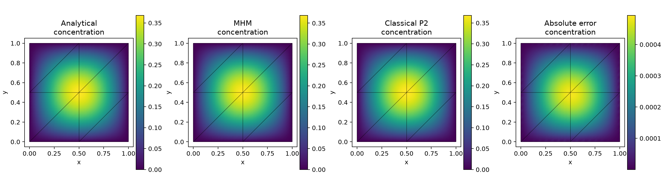
The same macro mesh is visible on all analytical, numerical and error panels. Macrocells retain their independent incident values.

7. Finish with first-order temporal convergence

Keep the above spatial approximation fixed and integrate to \(t=1\) with \(\Delta t=0.1,0.05,0.025,0.0125,0.00625\). The final consecutive physical concentration error ratios must approach the first-order backward-Euler target while remaining above the fixed spatial floor. Measured consecutive orders are \(1.0266\), \(1.0135\), \(1.0065\) and \(0.9996\); the final concentration \(L^2\) error is \(2.9934\times10^{-5}\). Condensed global compatibility residuals remain below \(1.24\times10^{-15}\). Both error curves and measured orders are plotted; a reference slope alone is not evidence of that order.

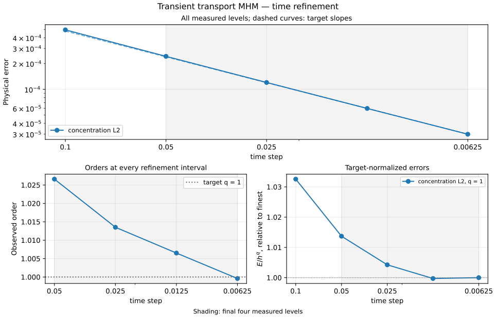
This experiment establishes the smooth temporal order of the displayed scheme; heterogeneous geometry, transport-dominated layers and monotonicity need separate assessments. The spatial study below qualifies the smooth spatial approximation independently. See the transport gallery for the other current physical studies.

The final provenance cell reads the executed notebook file, rather than expecting it inside the support archive. The public runner supplies PYMHM_NOTEBOOK_SOURCE. For manual execution, save the downloaded notebook as transient_variational.ipynb in the working directory. If you rename or move it, set PYMHM_NOTEBOOK_SOURCE to its path before running this cell. A checkout also supports its ordinary notebooks/transport/transient_variational.ipynb location.

source_file = Path(os.environ.get("PYMHM_NOTEBOOK_SOURCE", "transient_variational.ipynb"))
if not source_file.is_file() and "PYMHM_NOTEBOOK_SOURCE" not in os.environ:
    source_file = Path.cwd()/"notebooks/transport/transient_variational.ipynb"
source_bytes = source_file.read_bytes()
source_notebook = json.loads(source_bytes)
scientific_cells = [
    {"cell_type": cell["cell_type"],
     "source": "".join(cell["source"])
               if isinstance(cell["source"], list) else cell["source"]}
    for cell in source_notebook["cells"]
    if "pymhm-companion-bootstrap" not in cell.get("metadata", {}).get("tags", [])
]
scientific_bytes = json.dumps(
    scientific_cells, ensure_ascii=False, sort_keys=True, separators=(",", ":")
).encode("utf-8")
study["source_notebook_sha256"] = hashlib.sha256(source_bytes).hexdigest()
study["scientific_cells_sha256"] = hashlib.sha256(scientific_bytes).hexdigest()

The first digest identifies the literal acquired source bytes. The second identifies every scientific and explanatory cell, excluding only the generated installer tagged pymhm-companion-bootstrap. Outputs and execution counts are excluded from that second identity; the equations and their parameters remain part of it.

8. Define a spatial study with negligible time truncation

For the same diffusion, capacity, advection and reaction, choose

\[ \begin{aligned} c_*(t,x,y)&=t\phi(x,y), &\phi(x,y)&=\sin(\pi x)\sin(\pi y),\\ f(t,x,y)&=\phi+t\left[(2\pi^2+\tfrac12)\phi +\beta\cdot\nabla\phi\right]. \end{aligned} \]

Initial concentration and exterior concentration are zero. Backward Euler differentiates the exact linear-time concentration without truncation error; a halved time step additionally checks the influence of the discrete initial and spatial projection. The fixed-step spatial study uses \(\Delta t=0.01\) and \(T=0.5\). This is a new explicitly stated smooth analytical case, rather than a transient reproduction of a steady paper table.

In the spatial notebook, declare the continuous mass and operator with UFL before writing the local step and global moment equation:

def volume_forms(domain,c,v):
    x = ufl.SpatialCoordinate(domain)
    beta = ufl.as_vector((0.25,-0.5))
    phi = ufl.sin(np.pi*x[0])*ufl.sin(np.pi*x[1])
    grad_phi = ufl.grad(phi)
    dx = ufl.Measure("dx",domain=domain,metadata={"quadrature_degree":12})
    mass = c*v*dx
    operator = (ufl.inner(ufl.grad(c),ufl.grad(v))+0.5*c*v
                +0.5*(ufl.dot(beta,ufl.grad(c))*v-c*ufl.dot(beta,ufl.grad(v))))*dx
    initial_source = phi*v*dx
    linear_source = ((2*np.pi**2+0.5)*phi+ufl.dot(beta,grad_phi))*v*dx
    return mass,operator,initial_source,linear_source

Choose macro resolution \(n\), local \(P_2\) concentration on refinement two, unsplit scalar \(P_1\) traces and one retained mean. The retained constant is a coarse coordinate, not a kernel of the positive mass/reaction operator. Local pairings are \(b=\langle\lambda,v\rangle\) and \(c=-\langle\mu,c\rangle\), exactly as in the preceding temporal formulation. Assemble the same operator once and update loads as

\[ F_K^{m+1}=F_{0,K}+t_{m+1}F_{1,K}+M_Kc_K^m/\Delta t. \]

The spatial notebook assembles this explicitly declared family on an \(8\times8\) macro grid and compares the reconstructed concentration with the analytical field and independently assembled conforming P2 solution on a \(64\times64\) global grid. The actual macro mesh is visible on every panel.

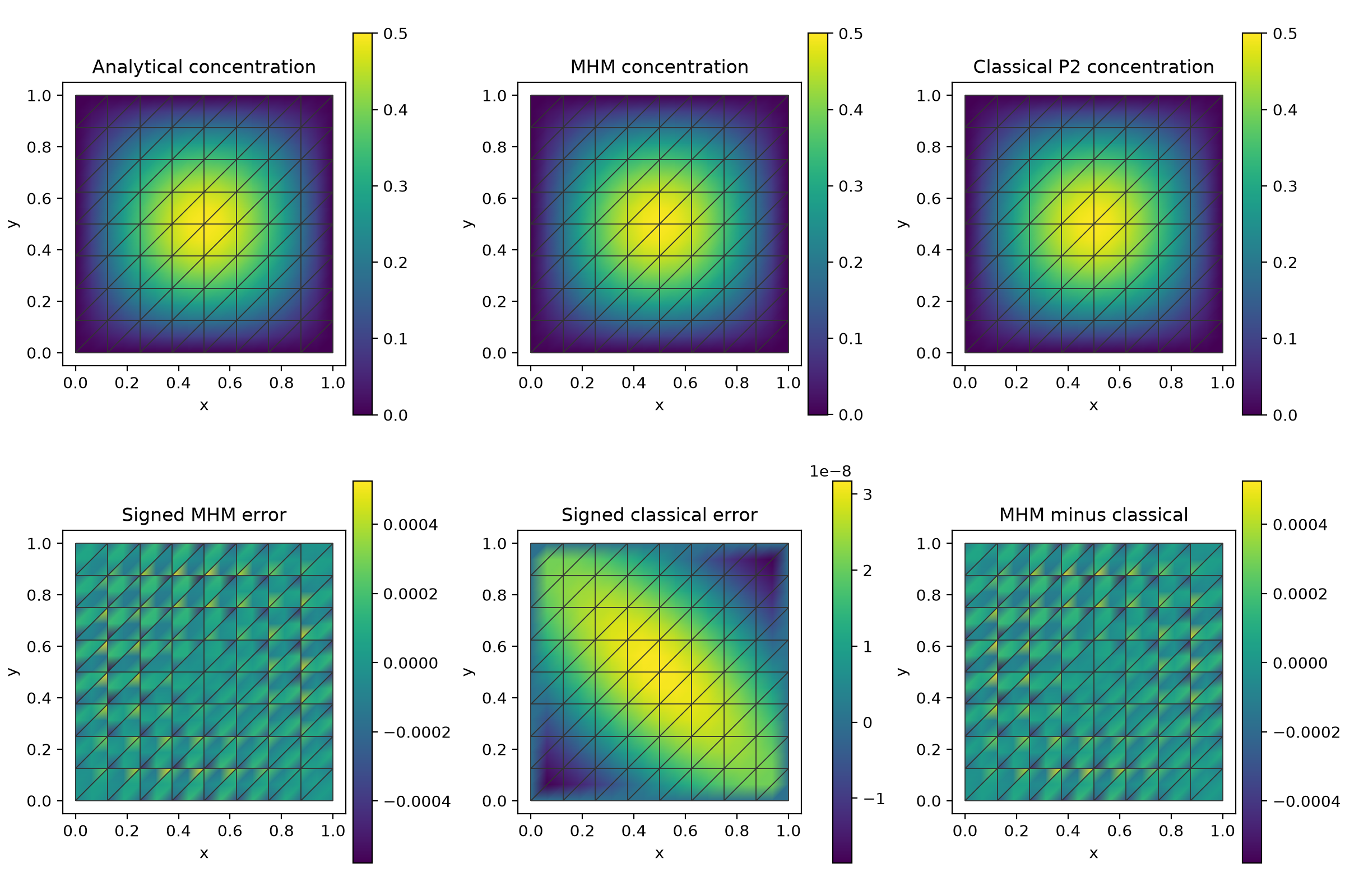
The concentration and broken gradient are integrated independently with quadrature orders six and eight; original physical rows are checked throughout the march.

The separately assembled conforming global \(P_2\) baseline uses the same UFL operator, source, zero exterior data, \(\Delta t=0.01\) and \(T=0.5\):

Classical mesh	Concentration \(L^2\)	Broken gradient \(L^2\)
\(32\times32\)	\(4.299\times10^{-6}\)	\(1.055\times10^{-3}\)
\(64\times64\)	\(5.376\times10^{-7}\)	\(2.638\times10^{-4}\)
\(128\times128\)	\(6.721\times10^{-8}\)	\(6.597\times10^{-5}\)

Its analytical errors show concentration order three and gradient order two. Halving the time step on the finest reference changes its concentration error by less than \(4\times10^{-8}\) relatively; the gradient error agrees to the reported precision. Thus the classical baseline has its own refinement control, rather than being declared exact because its mesh is fine.

The multiscale controls distinguish the condensed global compatibility residual from the original uncondensed local equations. A separate observer checks all original concentration blocks and global weak rows at every step on resolutions 4, 16 and 48, using eight spawn processes for local assembly. At resolution 48, the largest original relative residual is \(1.31\times10^{-13}\) and the largest local block backward error is \(1.93\times10^{-16}\). These algebraic diagnostics accompany the independently integrated physical concentration and gradient errors.

9. Compare the spatial target with its precise literature estimate

Araya et al. (2024), Section 2.3 assumption (A2), permits \(k=\ell+1\) in two dimensions with one refinement of the local triangulation. Here \(k=2\), \(\ell=1\), and local refinement two supplies that enrichment. Uniformly elliptic diffusion, nonnegative effective reaction, regular macroelements and smooth scalar and half-advection flux satisfy the hypotheses of Theorems 2 and 3. Their estimate (23) is

\[ \lVert c-c_h\rVert_V \le C\left(H^{\ell+1} \lvert-\nabla c+\tfrac12\beta c\rvert_{\ell+1} +h^k\lvert c\rvert_{k+1}\right). \]

Refining the macro grid and its proportionate local meshes therefore targets broken energy/gradient order two. The cited results concern stationary RAD problems; here they provide spatial targets for the elliptic operator of each backward-Euler step. The fixed-time numerical study and its separate time-step controls qualify this transient case; they do not establish a uniform-in-time parabolic error theorem. The separate concentration \(L^2\) curve measures additional accuracy; this RAD theorem does not itself assert an extra scalar \(L^2\) order. It is labeled observed, rather than attributing a stronger unproved estimate to that theorem.

The complete spatial sequence is \(n=4,8,16,24,32,48\). Its final four levels give the following three consecutive intervals, using their actual macro diameters rather than assuming every refinement is dyadic:

Physical observable	Reference order	Last three orders	Maximum/minimum of \(E/H^q\)
Concentration \(L^2\)	observed 3	2.9777, 2.9846, 2.9893	1.0180
Broken gradient \(L^2\)	2	1.9969, 1.9979, 1.9986	1.0024

Halving the MHM time step on resolution 48 changes the concentration and gradient errors by relative amounts \(2.47\times10^{-11}\) and \(1.27\times10^{-12}\). The independently refined classical reference and these time controls are attributed separately in the numerical record.

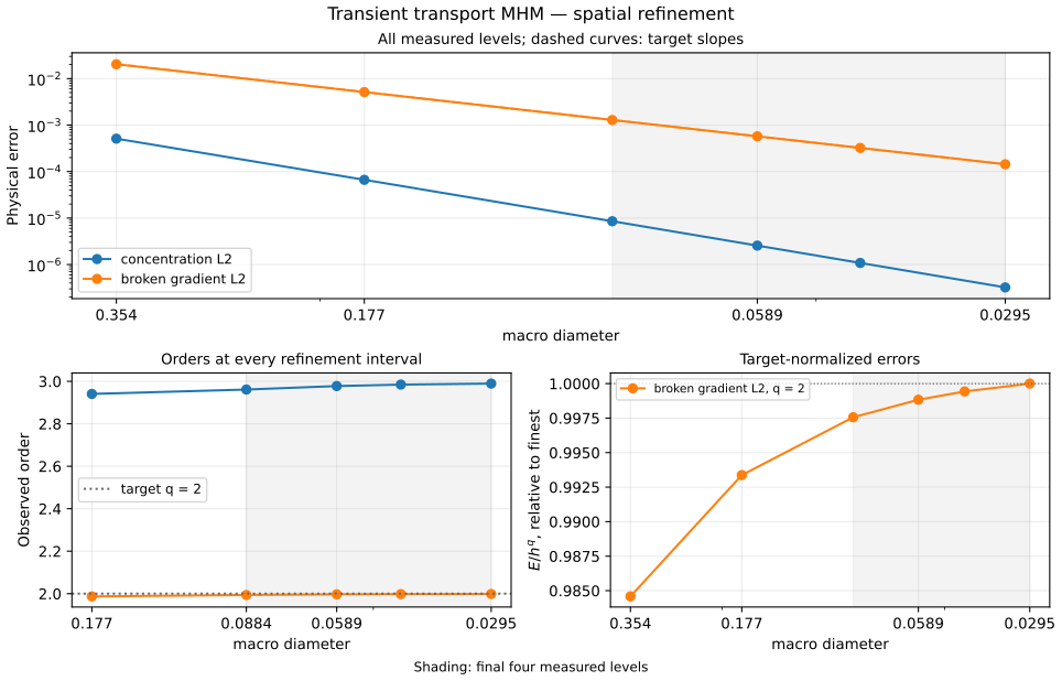
The spatial and temporal figures retain every measured level. Their final four-level windows are fixed by the end of each sequence; the last three consecutive rates and \(E/h^q\) variation assess a stable tail, not a selected single slope.

References

• Christopher Harder, Diego Paredes and Frédéric Valentin (2015). On a Multiscale Hybrid-Mixed Method for Advective-Reactive Dominated Problems with Heterogeneous Coefficients. Multiscale Modeling & Simulation 13(2), 491–518. DOI: 10.1137/130938499.
• Rodolfo Araya, Fabrice Jaillet, Diego Paredes and Frédéric Valentin (2024). Generalizing the multiscale hybrid-mixed method for reactive-advective-diffusive equations. Computer Methods in Applied Mechanics and Engineering 428,
• DOI: 10.1016/j.cma.2024.117089.