Robin MH
Open the step-by-step notebook · Download notebook
We write the Robin weak equations directly in UFL. Our independently manufactured data are \(p=\sin(2\pi x)\sin(2\pi y)\), \(K=I\), \(f=8\pi^2p\), and homogeneous exterior pressure. Follow meshes → local forms → global forms → assemble → solve → physical fields.
The modified multiplier is \(\lambda_T=(q-p\sigma)\cdot n_T\), where \(q=-\nabla p\) and \(\sigma=\nu(x-x_0)/2\). Consequently this multiplier cannot be plotted or tested as \(q\cdot n_T\). The method follows Barrenechea, Gomes and Paredes (2024).
import numpy as np
import matplotlib.pyplot as plt
import ufl
from pymhm import (
    Equation, FaceSpace, LocalContext, MeshHierarchy, SkeletonSpace, TriangleMesh,
    assemble, bind_interface, bind_problem, columns, solve,
)
from threadpoolctl import threadpool_limits


def exact_pressure(points: np.ndarray) -> np.ndarray:
    """Analytical pressure; it vanishes on every exterior edge."""
    return np.sin(2 * np.pi * points[:, 0]) * np.sin(2 * np.pi * points[:, 1])


def exact_gradient(points: np.ndarray) -> np.ndarray:
    """Independently differentiated physical pressure gradient."""
    x, y = 2 * np.pi * points.T
    return 2 * np.pi * np.column_stack((np.cos(x) * np.sin(y), np.sin(x) * np.cos(y)))


def source(points: np.ndarray) -> np.ndarray:
    """Negative Laplacian computed independently of the discrete operator."""
    return 8 * np.pi**2 * exact_pressure(points)
1. Define macro, local and interface spaces
The hierarchy owns mesh association. The interface binding owns geometric incidence and numbering; variational signs are declared separately.
macro = TriangleMesh.unit_square(2)
local_meshes = tuple(macro.submesh(cell, 2) for cell in range(len(macro.cells)))
hierarchy = MeshHierarchy(macro, local_meshes)
skeleton = SkeletonSpace(macro, tuple(FaceSpace.uniform(1) for _ in macro.faces))
interface = bind_interface(skeleton, convention="normal")
2. Declare the local Robin equations
Choose \(x_0=(0,0)\) and \(\nu=1/4\). On this unit-square problem, \(R=\sqrt{2}/2\) gives the admissible sufficient bound \(\nu\le 1/(4R^2)=1/2\). The Robin operator has no constant kernel: it retains no pressure mean. The global test remains the independent negative pressure trace pairing.
def local_equations(local: LocalContext):
    """Declare Robin diffusion and its independent pressure trace test."""
    space = local.native_space(degree=3)
    p, v = ufl.TrialFunction(space.space), ufl.TestFunction(space.space)
    x = ufl.SpatialCoordinate(space.mesh)
    dx = ufl.Measure("dx", domain=space.mesh, metadata={"quadrature_degree": 12})
    forcing = 8 * np.pi**2 * ufl.sin(2 * np.pi * x[0]) * ufl.sin(2 * np.pi * x[1])
    ds = ufl.Measure("ds", domain=space.mesh, metadata={"quadrature_degree": 12})
    normal = ufl.FacetNormal(space.mesh)
    sigma = 0.25 * x / 2
    local.field("pressure", space)
    return local.equations(
        a=ufl.inner(ufl.grad(p), ufl.grad(v)) * dx + ufl.dot(sigma, normal) * p * v * ds,
        L=forcing * v * dx,
        b=local.trace_pairings(lambda phi, ds: phi * v * ds),
        c=local.trace_pairings(lambda phi, ds: -phi * p * ds, axis="rows"),
    )
3. Declare global pressure continuity and boundary moments
The trace maps carry canonical incidence. The negative sign is the mathematical global-test convention. Zero retained coordinates reflect the invertible local Robin operator.
def global_equation(global_context):
    """Supply the weak Dirichlet moments in the bound interface layout."""
    boundary, fixed = global_context.boundary_data(0.0, order=8)
    assert not fixed
    return Equation(0, global_context.trace_load(-boundary))


problem = bind_problem(hierarchy, interface, local_equations,
                       global_equation=global_equation, retained=0)
4. Assemble and solve
Assembly solves the independent local equations and sums their interface contributions. Solving reconstructs named local fields in their executed coefficient bases.
with threadpool_limits(1):
    system = assemble(problem)
    coefficients = solve(system)
pressure_fields = coefficients.field("pressure")
5. Integrate physical errors
Pressure and its broken gradient are integrated separately with positive order-12 quadrature. No algebraic residual is used as a substitute for these errors.
from pymhm.fem.scalar.operators import triangle_quadrature
bary, weights = triangle_quadrature(12)
pressure_error, gradient_error = 0.0, 0.0
for fine, field in zip(local_meshes, pressure_fields, strict=True):
    points = np.einsum("qi,tia->tqa", bary, fine.points[fine.cells])
    flat = points.reshape(-1, 2)
    ep = (field.evaluate(flat) - exact_pressure(flat)).reshape(points.shape[:2])
    eg = (field.gradient(flat) - exact_gradient(flat)).reshape(*points.shape[:2], 2)
    pressure_error += np.einsum("t,q,tq->", fine.areas, weights, ep**2)
    gradient_error += np.einsum("t,q,tq->", fine.areas, weights, np.sum(eg**2, axis=-1))
print({"original_equation_residual": coefficients.raw_residual,
       "pressure_L2": float(np.sqrt(pressure_error)),
       "broken_gradient_L2": float(np.sqrt(gradient_error))})
assert coefficients.raw_residual < 1e-10
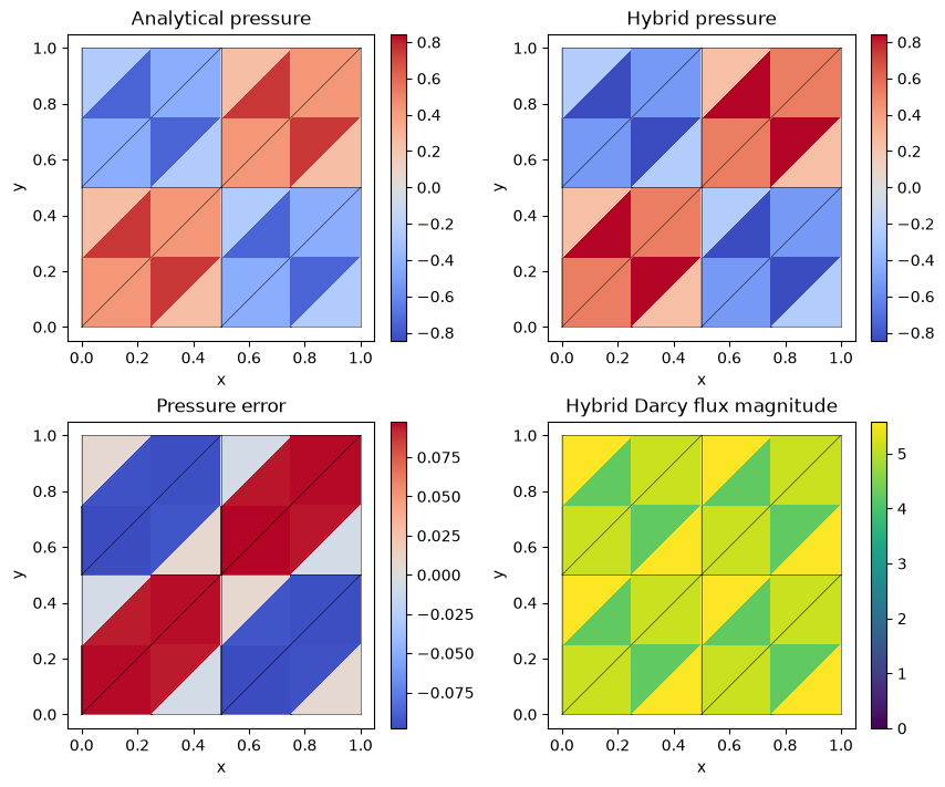
{'original_equation_residual': 1.4784624037949213e-16, 'pressure_L2': 0.12338705246283269, 'broken_gradient_L2': 1.7942089859434043}
6. Plot analytical, numerical and error fields
Independent local panels retain one-sided values. Every panel shows the actual macro partition.
fig, axes = plt.subplots(2, 2, figsize=(8.5, 7), layout="constrained")
all_exact, all_values, panels = [], [], []
for fine, field in zip(local_meshes, pressure_fields, strict=True):
    points = fine.points[fine.cells].mean(axis=1)
    exact, values = exact_pressure(points), field.evaluate(points)
    flux_magnitude = np.linalg.norm(-field.gradient(points), axis=1)
    panels.append((fine, exact, values, flux_magnitude))
    all_exact.extend(exact)
    all_values.extend(values)
common = max(np.max(np.abs(all_exact)), np.max(np.abs(all_values)))
error_max = max(np.max(abs(values - exact)) for _, exact, values, _ in panels)
flux_max = max(np.max(flux) for _, _, _, flux in panels)
titles = ("Analytical pressure", "Hybrid pressure", "Pressure error", "Hybrid Darcy flux magnitude")
for index, (ax, title) in enumerate(zip(axes.flat, titles, strict=True)):
    for fine, exact, values, flux in panels:
        value = (exact, values, values - exact, flux)[index]
        limit = (common, common, error_max, flux_max)[index]
        artist = ax.tripcolor(*fine.points.T, fine.cells, facecolors=value,
                             vmin=0.0 if index == 3 else -limit,
                             vmax=limit, cmap="viridis" if index == 3 else "coolwarm")
    for edge in macro.faces:
        ax.plot(*macro.points[edge].T, color="black", lw=0.5, alpha=0.7)
    ax.set(title=title, xlabel="x", ylabel="y", aspect="equal")
    fig.colorbar(artist, ax=ax)
plt.show()
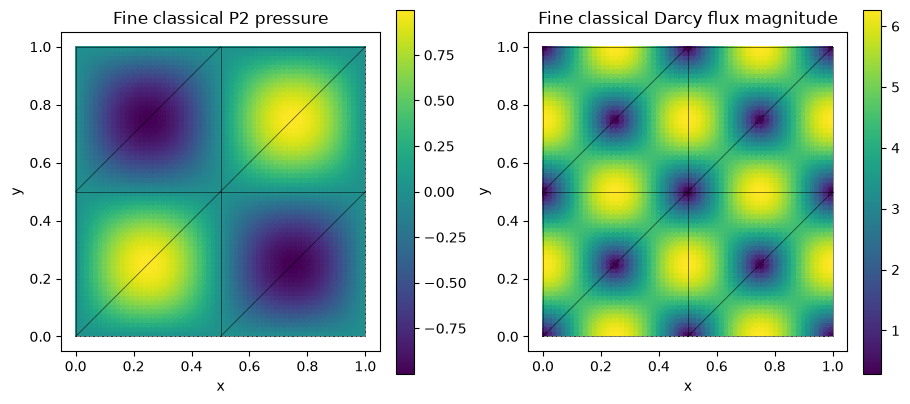
Independently refined classical primal Galerkin baseline
The classical baseline uses one globally conforming P2 space on independent 16×16, 32×32 and 64×64 triangular grids, with the same physical coefficient, source and boundary values:
The shared volume operator integrates this already stated form. The explicit essential lifting \(A_{ff}p_f=f_f-A_{fb}p_D\) selects its classical boundary values. Check this reference's own errors before comparing fields. The multiscale solve above retains its simpler macro mesh and separate local spaces; it does not use this refined global grid. An exactly representable polynomial has roundoff-level classical errors on all three grids.
from threadpoolctl import threadpool_limits
from pymhm.fem.scalar.triangle import scalar_operators, nodal_space, tabulate
from pymhm.fem.scalar.operators import triangle_quadrature
from pymhm.linalg.linear import solve_linear

classical_rows = []
bary, weights = triangle_quadrature(12)
for resolution in (16, 32, 64):
    reference_mesh = TriangleMesh.unit_square(resolution)
    A, _, forcing = scalar_operators(reference_mesh, 2, diffusion=1.0, source=source, order=12)
    dofs, nodes = nodal_space(reference_mesh, 2)
    boundary = np.flatnonzero(np.any(np.isclose(nodes, 0.0) | np.isclose(nodes, 1.0), axis=1))
    free = np.setdiff1d(np.arange(len(nodes)), boundary)
    reference_pressure = np.zeros(len(nodes))
    reference_pressure[boundary] = exact_pressure(nodes[boundary])
    rhs = forcing[free] - A[free][:, boundary] @ reference_pressure[boundary]
    with threadpool_limits(1):
        reference_pressure[free] = solve_linear(A[free][:, free], rhs)
    _, _, basis, gradient, _ = tabulate(reference_mesh, 2, bary)
    points = np.einsum("qi,tia->tqa", bary, reference_mesh.points[reference_mesh.cells])
    difference = reference_pressure[dofs] @ basis.T - exact_pressure(points.reshape(-1, 2)).reshape(points.shape[:2])
    error = float(np.sqrt(reference_mesh.areas @ (difference**2 @ weights)))
    classical_rows.append({"resolution": resolution, "elements": len(reference_mesh.cells),
                           "pressure_L2": error})
for row in classical_rows:
    print(row)
# Polynomial patches can be exactly represented, in which case all levels are
# at roundoff. Otherwise verify the classical reference's own refinement.
assert (max(row["pressure_L2"] for row in classical_rows) < 1e-10
        or all(b["pressure_L2"] < a["pressure_L2"] for a, b in zip(classical_rows, classical_rows[1:])))
centers = reference_mesh.points[reference_mesh.cells].mean(axis=1)
_, _, center_basis, center_gradient, _ = tabulate(reference_mesh, 2, np.full((1, 3), 1/3))
reference_values = (reference_pressure[dofs] @ center_basis.T)[:, 0]
reference_flux = -np.einsum("ti,tqia->tqa", reference_pressure[dofs], center_gradient)[:, 0]
fig, axes = plt.subplots(1, 2, figsize=(9, 4), layout="constrained")
for ax, values, title in zip(axes, (reference_values, np.linalg.norm(reference_flux, axis=1)),
                             ("Fine classical P2 pressure", "Fine classical Darcy flux magnitude"), strict=True):
    artist = ax.tripcolor(*reference_mesh.points.T, reference_mesh.cells, facecolors=values, cmap="viridis")
    for edge in macro.faces:
        ax.plot(*macro.points[edge].T, color="black", lw=0.5, alpha=0.7)
    ax.set(title=title, xlabel="x", ylabel="y", aspect="equal")
    fig.colorbar(artist, ax=ax)
plt.show()
{'resolution': 16, 'elements': 512, 'pressure_L2': 0.0005479034106938733}
{'resolution': 32, 'elements': 2048, 'pressure_L2': 6.873255317566801e-05}
{'resolution': 64, 'elements': 8192, 'pressure_L2': 8.600387223616975e-06}
7. Keep Robin and local refinement errors distinct
The smooth refinement uses the data of section 4.1, equation (4.1), in Barrenechea, Gomes and Paredes (2024): identity diffusion on the unit square, homogeneous exterior pressure, and independently differentiated fields
The L-shaped macroelements partition the square; the physical domain has no reentrant corner. Keep P3 local pressure, two local subdivisions, P1 Robin traces and \(\nu=1/4\) fixed throughout macro refinement. These data differ from the lower-frequency field illustration above; the variational equations are unchanged.
Corollary 2.7 separates the skeletal and local Galerkin contributions:
Assumption A1, matching regularly refined local partitions, and the stated pressure/modified-flux regularity belong to this estimate. With \(\ell=1\), \(k=3\) and fixed \(h/H\), the second-order contribution governs the physical-flux error. Pressure order three is a numerical observation for these smooth data. The Robin multiplier is not the physical Darcy flux: the volume error uses \(q=-K\nabla p\), rather than multiplier coefficients.
Recompute orders from the numerical record
For successive physical errors at the actual refinement sizes, compute
The cell below reads the attributed record and recomputes the complete table, consecutive orders, final-four-level fitted slope and plot. It does not choose a PDE or rerun the acquisition. For a justified target \(q\), the maximum/minimum of \(E/h^q\) over the final four levels measures stabilization of its amplitude. Pressure orders reported as observations are kept separate from theorem targets.
import json
from IPython.display import Markdown, display
from examples.tutorial_convergence import refinement_series, asymptotic_summary, plot_method_series
refinement_record = ROOT / 'examples/results/mh/comparison.json'
refinement_data = json.loads(refinement_record.read_text(encoding='utf-8'))
refinement_rows = [refinement_row for refinement_row in refinement_data['smooth'] if refinement_row['mesh'] == 'L-polygons' and refinement_row['trace_degree'] == 1]
refinement_error_keys = {'pressure L2': 'pressure_error_l2', 'physical Darcy flux L2': 'flux_error_l2'}
refinement_targets = {'physical Darcy flux L2': 2.0}
refinement_rows = sorted(refinement_rows, key=lambda refinement_row: refinement_row['macro_diameter'], reverse=True)
refinement_sizes = np.asarray([refinement_row['macro_diameter'] for refinement_row in refinement_rows])
refinement_field_errors = {refinement_field: np.asarray([refinement_row[refinement_key] for refinement_row in refinement_rows]) for refinement_field, refinement_key in refinement_error_keys.items()}
refinement_orders = {refinement_field: np.log(refinement_values[:-1] / refinement_values[1:]) / np.log(refinement_sizes[:-1] / refinement_sizes[1:]) for refinement_field, refinement_values in refinement_field_errors.items()}
refinement_header = ['Refinement size'] + [refinement_column for refinement_field in refinement_error_keys for refinement_column in (refinement_field, 'Order')]
refinement_lines = [' | '.join(refinement_header), ' | '.join(['---'] * len(refinement_header))]
for refinement_index, refinement_size in enumerate(refinement_sizes):
    refinement_values = [f'{refinement_size:.6g}']
    for refinement_field in refinement_error_keys:
        refinement_values.extend([f'{refinement_field_errors[refinement_field][refinement_index]:.6e}', '—' if refinement_index == 0 else f'{refinement_orders[refinement_field][refinement_index - 1]:.3f}'])
    refinement_lines.append(' | '.join(refinement_values))
display(Markdown('\n'.join(refinement_lines)))
refinement_series_data = refinement_series(refinement_record, refinement_rows, 'macro_diameter', refinement_error_keys, refinement_targets, method='robin-mh', spaces='P3/r2 locals; P1 Robin trace; nu=1/4', rate_provenance='Barrenechea, Gomes and Paredes (2024), Corollary 2.7: energy order two under Assumption A1, matching regularly refined local partitions and the stated pressure/modified-flux regularity; pressure order three observed separately.', refinement='macro diameter', root=ROOT)
print({'record': refinement_series_data['record'], 'sha256': refinement_series_data['sha256']})
for refinement_field, refinement_summary in asymptotic_summary(refinement_series_data).items():
    print(refinement_field, {'last_three_orders': [round(refinement_order, 3) for refinement_order in refinement_summary['orders']], 'fitted_order': round(refinement_summary['fitted_order'], 3), 'target': refinement_summary['target'], 'normalized_amplitude_ratio': refinement_summary.get('amplitude_ratio')})
plot_method_series(refinement_series_data)
plt.show()
| Refinement size | pressure L2 | Order | physical Darcy flux L2 | Order |
|---|---|---|---|---|
| 0.600925 | 1.815189e-01 | — | 1.080378e+01 | — |
| 0.300463 | 3.378326e-02 | 2.426 | 3.009670e+00 | 1.844 |
| 0.150231 | 4.269770e-03 | 2.984 | 7.249964e-01 | 2.054 |
| 0.0751157 | 5.247353e-04 | 3.024 | 1.769622e-01 | 2.035 |
| 0.0375578 | 6.522051e-05 | 3.008 | 4.392428e-02 | 2.010 |
{'record': 'examples/results/mh/comparison.json', 'sha256': '0e49ca0d9f39bf10d94b911b0cd64624194652a5932222bac1f1b00fa0086f39'}
pressure L2 {'last_three_orders': [2.984, 3.024, 3.008], 'fitted_order': 3.007, 'target': None, 'normalized_amplitude_ratio': None}
physical Darcy flux L2 {'last_three_orders': [2.054, 2.035, 2.01], 'fitted_order': 2.033, 'target': 2.0, 'normalized_amplitude_ratio': 1.070617413814136}
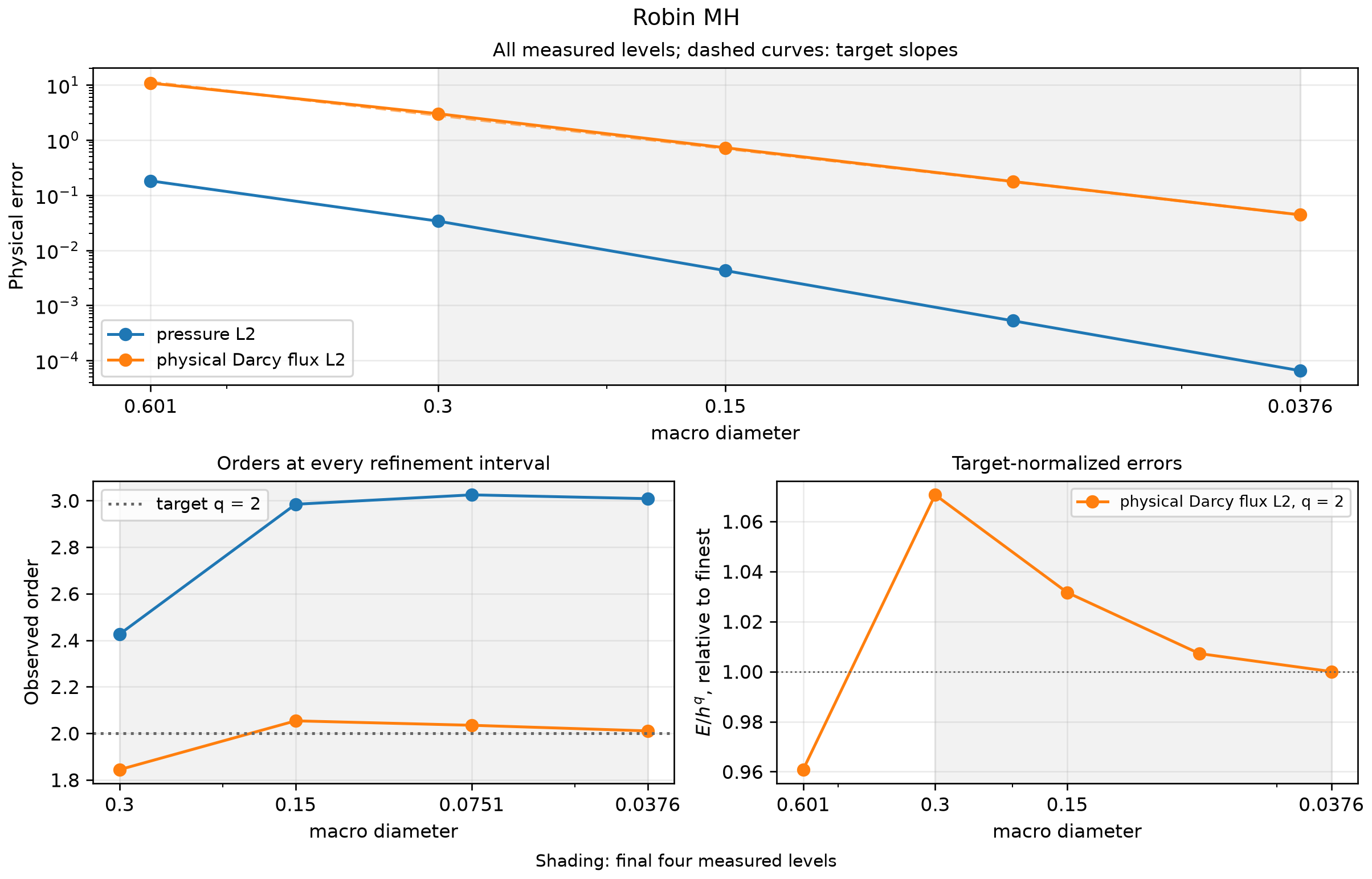
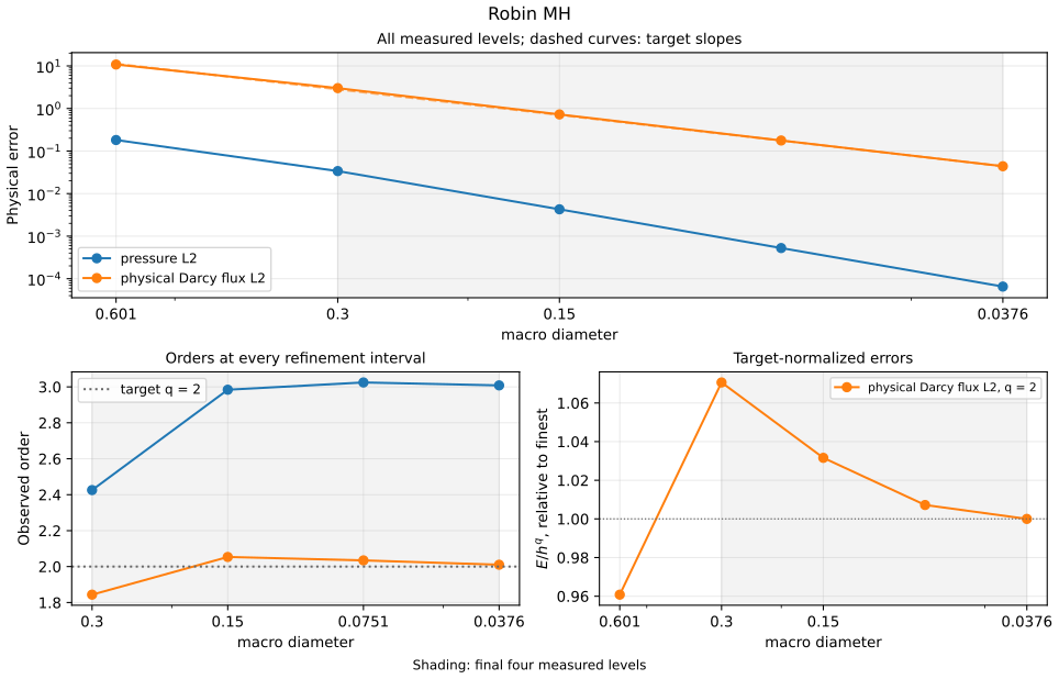
All coarse and fine measurements are retained; shading covers the final four levels. The publication figure is generated from the same attributed record read by the notebook, separately from its embedded field plots. See convergence plot conventions for the target curves, interval orders and normalized amplitudes.
Reproduce this tutorial
Open the notebook linked at the top. Its checksum-verified companion supplies inspectable support files and the refinement record. The notebook executes the variational workflow; its convergence cell reads the record and recomputes the table and plot, without rerunning the full acquisition. Use the installation guide for notebook, plotting and native-backend requirements. From a source checkout:
References
- Gabriel R. Barrenechea, Antonio Tadeu A. Gomes, and Diego Paredes (2024). A Multiscale Hybrid Method. SIAM Journal on Scientific Computing 46(3), A1628–A1657. DOI: 10.1137/22M1542556.