MsHHO: cell and face moment reconstruction

MsHHO means Multiscale Hybrid High-Order. solve_mshho constructs its cell and face pressure moments from constrained local energy minimization. MsHHO is the macro discretization: after eliminating cell moments, it solves a global system in shared face-pressure moments. The local reconstructions use conforming finite elements on fine submeshes of the macrocells; the implemented local discretization is not an HHO method on a second mesh.

It uses finite conforming Galerkin realizations of the projected-source formulation (4.6) and reconstructed-source formulation (5.1) of Chaumont-Frelet et al. (2022). The article establishes an equivalence theorem with exactly solved local problems; it does not provide a numerical benchmark table. The comparisons here measure a finite Galerkin analogue against the MHM construction in PyMHM. They do not reproduce the exact local multiscale spaces of that theorem. Remark 7.7 describes particular second-level multiscale or local HHO spaces for two-level equivalence; an arbitrary conforming \(P_k\) local space does not automatically satisfy those hypotheses.

Spaces and source convention

The macrocell unknowns are moments against \(P_m(K)\), while each macroface has independent polynomial moments. The reconstructed field minimizes \(\int_K A\nabla v\cdot\nabla v\) subject to those cell and face moments. Its implementation uses a conforming local \(P_k\) discretization of that minimization. Cell moments are eliminated before assembling the global face operator. For the symmetric diffusion form, independent local moment constraints and physical Dirichlet elimination give a symmetric positive definite face operator in exact arithmetic. The assembled reduction retains the represented Galerkin operator \(R^TAR\), including its floating-point antisymmetry.

For source_variant="projected", the load uses the cellwise \(L^2\) projection of the source onto \(P_m(K)\). For source_variant="reconstructed", the original load acts on the reconstructed test function. Polynomial sources in \(P_m(K)\) give identical fields. Theorem 5.1 distinguishes the original MHM construction with a source in \(P_m(K)\) from its fully explicit projected-source construction for general \(L^2\) sources. Remark 5.3 relates the reconstructed-source variant to a corresponding approximate MHM source lifting; it does not identify it with an arbitrary full-source finite-element MHM solve. The face-only setting cell_degree=-1 uses the reconstructed-source variant, as in Remark 5.4; it is not the same method as MHM with a source lifting.

Lemma 4.2's \(H(\mathrm{div})\) property applies to the exact-local projected-source solution. Remark 5.3 explicitly states that the reconstructed-source variant can lose that property even with exact local solves. The broken finite Galerkin raw flux on this page therefore requires its own normal-continuity measurement.

The example helpers below are repository sources, supplied separately from the installed library. Open the corresponding notebook to acquire its verified companion, as described in the notebook guide.

from pymhm import FaceSpace, SkeletonSpace, TriangleMesh
from examples.formulations.application import moment_diffusion as solve_mshho

mesh = TriangleMesh.unit_square(4)
faces = tuple(FaceSpace.uniform(1) for _ in mesh.faces)
solution = solve_mshho(
    mesh, skeleton=SkeletonSpace(mesh, faces), cell_degree=1,
    degree=3, local_refinement=2, source=4.0,
)

Polygonal macrocells use solve_mshho_polygons with the same moment spaces and local energy minimization. Nonconvex L-shaped cells are included in the field equivalence tests.

Five-level analytical convergence

The unit-square problem uses \(A=I\), zero Dirichlet data, \(u=\sin(\pi x)\sin(\pi y)\) and \(f=2\pi^2u\). Both configurations use local \(P_3\) elements and two subdivisions of every macrotriangle edge. Macro spacing ranges from \(1\) to \(1/16\). Error quadrature is independent of assembly.

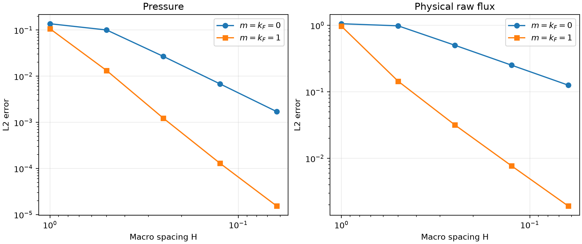
Five-level pressure and physical flux convergence

For \(m=k_F=0\) and \(m=k_F=1\), Theorem 6.3's ideal-space energy estimate has leading order one and two, respectively, under its source/conormal regularity and mesh hypotheses. It does not give the pressure \(L^2\) orders. The final measured pressure/raw-flux orders here are approximately 2.00/1.00 and 3.08/2.01, respectively. Local discretization remains part of the measured error.

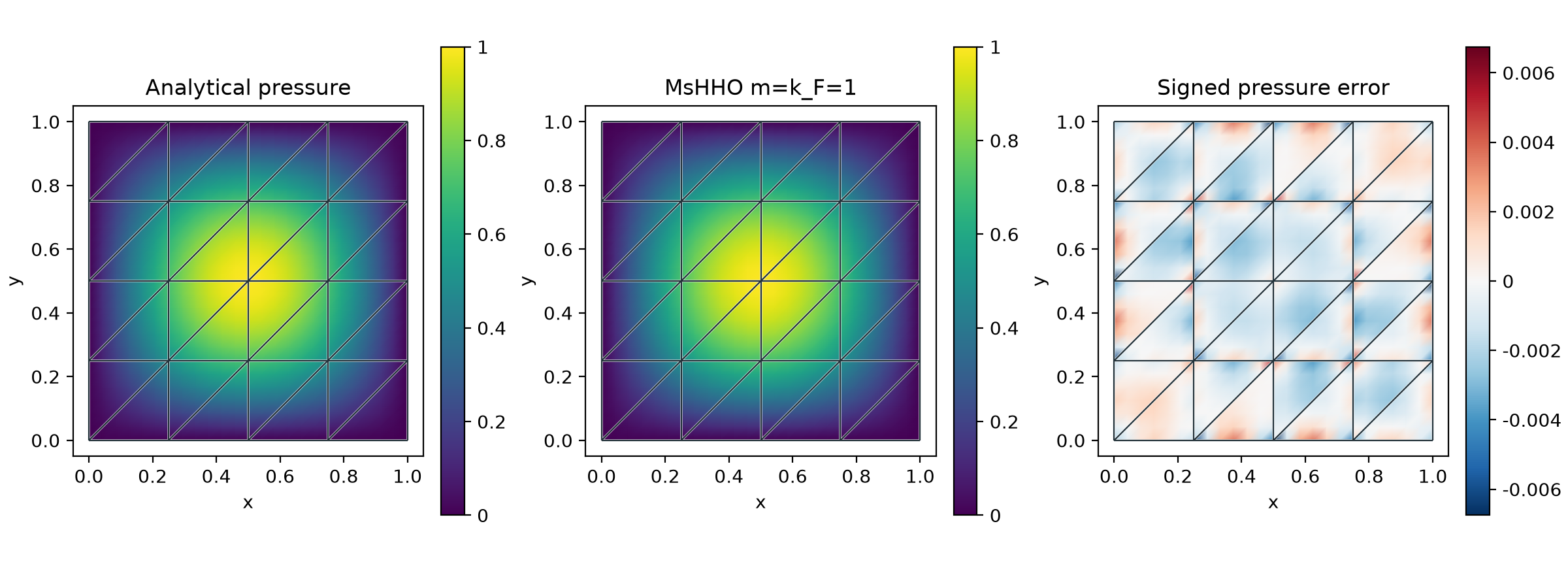
Analytical, reconstructed and error fields with the macro mesh

The panels use separate broken local fields, without smoothing macro interfaces. The error panel has its own symmetric scale. The plotted raw flux is not asserted to be globally \(H(\mathrm{div})\) conforming.

Equivalence and numerical precision

The polynomial-source comparison uses \(A=\mathrm{diag}(\kappa,1)\), \(f=4\), nonzero affine boundary data, local \(P_3\) and degree-one face/cell moments. The records include field differences and residuals for each \(\kappa\). For the shared assembled operator, the maximum relative nodal pressure difference through \(\kappa=10^6\) is \(4.36\times10^{-13}\). Both complete original saddle residuals are at most \(5.35\times10^{-12}\), with the original criterion \(10^{-10}\). MsHHO retains wider digits in its reconstructions, Galerkin reductions and moment coordinates. MHM uses wider local accumulation and two full original equation corrections, requested with hybrid_refinement_steps=2 and hybrid_refinement_min_steps=2. Factors remain binary64. The default minimum is zero, which permits stopping once the original residual criterion is met. The wider mode requires a platform whose longdouble has more mantissa bits than float64; an unsupported platform raises SolverUnavailableError.

The independently assembled comparison uses FEniCS Basix 0.9.0, revision 19555f5, through basix.finite_element and basix.polynomials. The executed comparison adapter assembles its geometry, cardinal bases, volume and face integrals independently. It shares the checked SciPy factorization and original-residual arithmetic with PyMHM. It uses all eight macrocells, the same local \(P_3\) spaces, materials, source, Dirichlet data and physical field norms. Pressure, raw gradient and Darcy flux differences meet the declared \(10^{-9}\) criterion at all four contrasts. The homogeneous Dirichlet control at \(\kappa=10^6\) also meets this criterion. A separate insertion into the other assembly's original saddle has residual about \(5.19\times10^{-9}\) at \(\kappa=10^6\), exceeding its declared \(10^{-10}\) criterion in both directions. The measured action of the difference between the two rounded operators explains this discrepancy. Joint certification of that insertion remains unresolved; field agreement and each assembly's own accepted equations are recorded separately. These finite-case checks do not establish a contrast-independent error bound or uniform inf-sup stability.

The compact record examples/results/mshho/native-verification.json identifies the executed binary and adapter digests, actual archived bases and coefficient vectors, quadrature controls, and each separate acceptance result. Field replay uses those archived bases and reproduces sampled fields and original rows bitwise with one and two BLAS threads. Coherent basis reordering preserves the physical fields; inconsistent reordering is rejected. The external solver sources and comparison tools are kept outside the package's release artifacts.

Run pixi run --locked -e notebooks verify-mshho to acquire and render the study. The numerical record is examples/results/mshho.json; compact algebraic, source-convention and polynomial-patch checks run in the test suite.

References

Théophile Chaumont-Frelet, Alexandre Ern, Simon Lemaire, and Frédéric Valentin (2022). Bridging the Multiscale Hybrid-Mixed and Multiscale Hybrid High-Order Methods, ESAIM: M2AN 56, 261–285. DOI: 10.1051/m2an/2021082.