Primal elasticity MHM

Follow meshes → local equations → global equations → assemble → solve → physical fields. We prescribe horizontal extension of a square containing a smooth oscillatory elastic material. The fine conforming reference is refined independently; it is not an exact solution.

Executable notebook

1. Define material, loading and scales

On the unit square, impose a one-percent horizontal extension on the whole exterior, with no body force:

\[ -\nabla\cdot\sigma=0,\qquad \sigma=2\mu\varepsilon(\boldsymbol u)+\lambda\operatorname{div}(\boldsymbol u)I, \qquad\boldsymbol u_D=(0.01x,0). \]

Here \(\varepsilon(\boldsymbol u)=(\nabla\boldsymbol u+\nabla\boldsymbol u^T)/2\). Use a smooth material with short wavelength and Lamé-modulus contrast \(e^3\simeq20.1\):

\[ \lambda(x,y)=\mu(x,y)=\exp\!\left(1.5\sin(16\pi x)\sin(16\pi y)\right). \]

The material wavelength is \(1/8\). Taking \(\lambda=\mu\) gives Poisson ratio \(1/4\) in plane strain, so this case isolates multiscale heterogeneity rather than near-incompressibility. The stiffness is uniformly positive on symmetric strains. Both methods solve the same tensor, domain and boundary values.

import numpy as np
import ufl
from pymhm import Equation, LocalEquations, MeshHierarchy, LocalContext, assemble, columns, bind_interface, bind_problem
from pymhm.meshes.triangle import TriangleMesh
from pymhm.fem.scalar.triangle import nodal_space
from pymhm.fem.scalar.operators import boundary_data
from pymhm.fem.traces.interval import FaceSpace, SkeletonSpace
from pymhm.execution.cpu import ExecutionConfig
from numpy.typing import NDArray
Array = NDArray[np.float64]

def micro_modulus(points: Array) -> Array:
    """Return smooth plane-strain Lamé values in [exp(-1.5),exp(1.5)], wavelength 1/8.

    Both lambda and mu equal this value, hence Poisson ratio is 1/4 and
    heterogeneity is separated from near-incompressibility and locking.
    """
    return np.exp(1.5 * np.sin(16 * np.pi * points[:, 0]) * np.sin(16 * np.pi * points[:, 1]))


def extension_boundary(points: Array) -> Array:
    """Prescribe a one-percent horizontal extension, with zero vertical displacement."""
    return np.column_stack((0.01 * points[:, 0], np.zeros(len(points))))

macro = TriangleMesh.unit_square(4)
local_degree, local_refinement, trace_segments = 3, 16, 4
skeleton = SkeletonSpace(
    macro, tuple(FaceSpace.uniform(1, trace_segments) for _ in macro.faces), components=2
)
print(
    {
        "macro_triangles": len(macro.cells),
        "material_wavelength": 1 / 8,
        "material_contrast": float(np.exp(3.0)),
        "local_degree": local_degree,
        "local_refinement": local_refinement,
        "trace_degree": 1,
        "trace_segments": trace_segments,
    }
)

2. Identify the kernel before solving

Integration by parts yields

\[ \int_T \left[2\mu\varepsilon(\boldsymbol u):\varepsilon(\boldsymbol v) +\lambda\operatorname{div}\boldsymbol u\operatorname{div}\boldsymbol v\right] -\langle\sigma\boldsymbol n_T,\boldsymbol v\rangle_{\partial T}=0. \]

Declare the skeletal multiplier \(\boldsymbol\lambda=-\sigma\boldsymbol n_F\): it is negative physical Cauchy traction in the unique macroface orientation. Thus the local equation is \(A_T\boldsymbol u+B_T\boldsymbol\lambda=0\), with the signed trace map \(B_T\).

The local energy has three exact rigid modes: translations \((1,0)\) and \((0,1)\), and centered rotation \((-(y-y_T),x-x_T)\). Their physical \(L^2\) moments select a unique response in the complement, while three retained coordinates represent the rigid component. We declare these modes, rather than infer them from a numerically rotated nullspace.

The trace contains the restrictions of rigid motions: degree one. The local degree is three. Harder, Madureira and Valentin (2016), Lemma 6.6 give the sufficient rule \(k\ge\ell+2\) for odd-degree traces on a single triangular local element. Our refined and segmented spaces differ from that single-element setting, so the rule alone is not their stability theorem. Segments align with the fine boundary and each covers four fine edges. We additionally check the rank of the actual trace pairing; an algebraic residual alone would not establish compatibility.

Weak-form term	Visible code
\(2\mu\varepsilon(u):\varepsilon(v)+\lambda\operatorname{div}u\operatorname{div}v\)	UFL expression a
\(\langle s_{TF}\lambda,v\rangle\)	local.trace_pairings(lambda phi, ds: inner(phi,v)*ds)
Rigid kernel	kernel
Physical rigid moments	columns of UFL linear forms
Global displacement continuity	independent UFL pairing -inner(phi,u)*ds, with axis="rows"
def rigid_modes(points: Array, center: Array) -> Array: """Return two translations and centered counterclockwise rotation, shape (n,2,3).""" modes = np.zeros((len(points), 2, 3)) modes[:, :, :2] = np.eye(2) modes[:, 0, 2] = -(points[:, 1] - center[1]) modes[:, 1, 2] = points[:, 0] - center[0] return modes

3. Translate each weak term into UFL

local.native_space binds the Basix element to this macrocell's fine mesh. The field declaration records the actual coefficient basis. Both trial and test trace pairings use the bound orientation.

def local_elasticity(local: LocalContext) -> LocalEquations:
    """Declare plane-strain UFL energy, negative Cauchy traction and rigid moments."""
    cell, fine = local.cell, local.mesh
    import basix
    import basix.ufl

    element = basix.ufl.element(
        "Lagrange",
        "triangle",
        local_degree,
        lagrange_variant=basix.LagrangeVariant.equispaced,
        shape=(2,),
    )
    binding = local.native_space(element)
    domain, space, mapping = binding.mesh, binding.space, binding.mapping
    u, v = ufl.TrialFunction(space), ufl.TestFunction(space)
    x = ufl.SpatialCoordinate(domain)
    mu = ufl.exp(1.5 * ufl.sin(16 * np.pi * x[0]) * ufl.sin(16 * np.pi * x[1]))
    lam = mu
    dx = ufl.Measure("dx", domain=domain, metadata={"quadrature_degree": 16})
    # This is exactly the physical energy written above.
    a = (
        2 * mu * ufl.inner(ufl.sym(ufl.grad(u)), ufl.sym(ufl.grad(v)))
        + lam * ufl.div(u) * ufl.div(v)
    ) * dx
    _, nodes = nodal_space(fine, local_degree)
    center = macro.points[macro.cells[cell]].mean(axis=0)
    portable_kernel = rigid_modes(nodes, center).reshape(-1, 3)
    kernel = binding.to_native(portable_kernel)
    rigid = (
        ufl.as_vector((1.0, 0.0)),
        ufl.as_vector((0.0, 1.0)),
        ufl.as_vector((-(x[1] - center[1]), x[0] - center[0])),
    )
    moments = columns(*(ufl.inner(v, mode) * dx for mode in rigid))
    local.field("displacement", binding)
    b = local.trace_pairings(lambda phi, ds: ufl.inner(phi, v) * ds)
    c = local.trace_pairings(lambda phi, ds: -ufl.inner(phi, u) * ds, axis="rows")
    return local.equations(
        a=a,
        L=np.zeros(len(mapping)),
        b=b,
        c=c,
        kernel=kernel,
        moments=moments,
        metadata=(fine, mapping),
    )

4. Impose global continuity and displacement data

The global weak equation imposes displacement-jump moments on interior macrofaces and prescribed displacement moments on the exterior. With \(C=-B^T\), its additional load is \(-\langle\boldsymbol\mu,\boldsymbol u_D\rangle_{\partial\Omega}\). Full displacement data remove the three global rigid ambiguities, so no additional physical gauge is required.

Only the macroface and three retained rigid coordinates per macroelement enter the global matrix. The local fields are recovered in their executed native basis, then mapped to the portable nodal representation for physical evaluation.

boundary, fixed = boundary_data(skeleton, extension_boundary, order=8)
hierarchy = MeshHierarchy(
    macro, tuple(macro.submesh(cell, local_refinement) for cell in range(len(macro.cells)))
)
problem = bind_problem(
    hierarchy,
    bind_interface(skeleton, convention="normal"),
    local_elasticity,
    global_equation=lambda global_problem: Equation(0, global_problem.trace_load(-boundary)),
    retained=3,
    fixed=fixed,
)
system = assemble(problem, execution=ExecutionConfig("serial", native_threads=1))
solution = system.solve()
displacement_fields = solution.field("displacement")
inspect_elasticity_solution(system, solution, macro)

5. Evaluate physical fields and the reference

The notebook evaluates the named displacement fields in their executed native bases, then assembles an independent conforming P2 reference on meshes 32, 64 and 128. It reports successive reference differences, displacement errors and Cauchy-stress errors separately. Analytical, numerical and error panels carry the actual macro mesh. Stress obtained from the primal gradient is a raw stress; it is not a mixed H(div) stress.

See the rendered heterogeneous fields.

6. Verify the smooth asymptotic rate

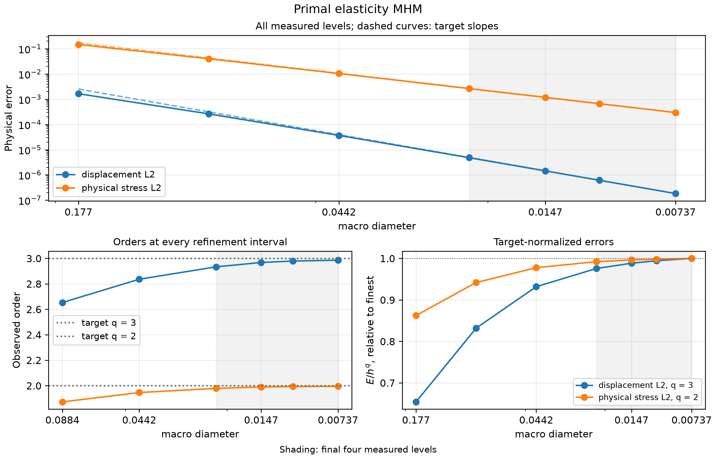
The heterogeneous example illustrates material resolution. Its rates cannot be inferred from a smooth constant-material theorem. The separate smooth manufactured study below keeps P3 displacement, P1 vector physical traction and one local triangle per macrocell, with a fixed homogeneous anisotropic positive-definite Kelvin tensor. It targets displacement order three and stress order two. The load is derived from the analytical displacement independently of assembly.

Vector SVG · Publication PDF

Observable	Expected order	Last three orders	Maximum/minimum of \(E/H^q\)
displacement \(L^2\)	3	2.9680, 2.9792, 2.9861	1.0249
physical stress \(L^2\)	2	1.9898, 1.9933, 1.9955	1.0079

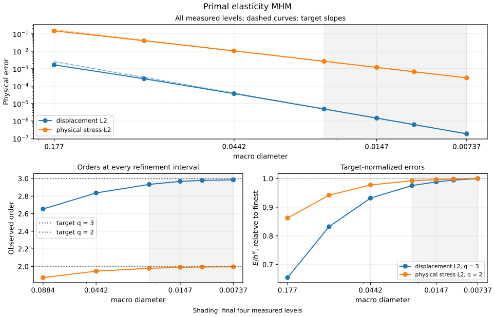
The complete sequence is \(n=8,16,32,64,96,128,192\). Its final four levels retain the actual non-dyadic macro diameters, so each consecutive order uses the exact logarithmic mesh ratio. Both target-normalized amplitudes flatten over the same three intervals; earlier coarse levels remain in the figure.

The degree choice uses the admissible odd trace degree from Harder, Madureira and Valentin (2016). Full exterior displacement removes global rigid ambiguities; every local translation and rotation moment is retained. This smooth estimate assumes the stated regular mesh family and displacement regularity. The extra displacement \(L^2\) order also requires the adjoint smoothing hypothesis in Theorem 5.2 and Corollary 6.4: the homogeneous Dirichlet dual solution \(w\) with \(L^2\) load \(e\) satisfies

\[ \lVert w\rVert_{H^2(\Omega)}\le C\lVert e\rVert_{L^2(\Omega)}. \]

Corollary 6.4 additionally retains the error from approximating the local lifting operators. Smoothness of the manufactured primal displacement alone does not establish this dual hypothesis. The measured third-order displacement tail is consistent with the conditional estimate; it does not give a material-independent rate for the preceding oscillatory example.

Norm integration uses independent quadrature orders 12 and 16. Their relative changes remain below \(3.7\times10^{-11}\) on the finest extension, with the original equation checks evaluated separately. The numerical record preserves each original row's input file and digest, including the current-source extensions. The notebook compares the field and stress through their independent physical norms, rather than using an algebraic residual as an error.

7. Refine a classical reference for the same smooth problem

For the smooth rate study in Step 6, an independently assembled conforming P3 reference uses the same unit square, anisotropic tensor, manufactured displacement and zero exterior data. In the orthonormal Kelvin convention, its material and exact displacement are

\[ C=\begin{pmatrix}5&1&0.4\\1&4&0.3\\0.4&0.3&2\end{pmatrix}, \qquad \boldsymbol u_{\mathrm{exact}}= \begin{pmatrix}\sin(\pi x)\sin(\pi y)\\\sin(2\pi x)\sin(\pi y)\end{pmatrix}. \]

The Kelvin strain is \((\varepsilon_{xx},\varepsilon_{yy}, \sqrt{2}\varepsilon_{xy})\). Multiplication by \(C\) gives \((\sigma_{xx},\sigma_{yy},\sqrt{2}\sigma_{xy})\), so converting back to the physical tensor counts both shear entries in its Frobenius norm. The conforming form has no skeletal multiplier or local rigid coordinates:

\[ \begin{aligned} V_h&\subset[H^1_0(\Omega)]^2,\\ \int_\Omega\sigma(\boldsymbol u_h):\varepsilon(\boldsymbol v_h) &=\int_\Omega\boldsymbol f\cdot\boldsymbol v_h \quad\text{for every }\boldsymbol v_h\in V_h,\\ \boldsymbol f&=-\nabla\cdot\sigma(\boldsymbol u_{\mathrm{exact}}). \end{aligned} \]

The following UFL definition differentiates the force independently of the analytical Hessian used in the MHM acquisition. Here space is the bound global vector P3 space and domain its mesh.

C = ufl.as_matrix(((5.0, 1.0, 0.4), (1.0, 4.0, 0.3), (0.4, 0.3, 2.0)))

def cauchy_stress(displacement):
    """Map orthonormal Kelvin strains back to the physical symmetric tensor."""
    strain = ufl.sym(ufl.grad(displacement))
    kelvin = ufl.as_vector((strain[0, 0], strain[1, 1], np.sqrt(2) * strain[0, 1]))
    stress = ufl.dot(C, kelvin)
    return ufl.as_matrix(
        ((stress[0], stress[2] / np.sqrt(2)), (stress[2] / np.sqrt(2), stress[1]))
    )

x = ufl.SpatialCoordinate(domain)
exact = ufl.as_vector(
    (ufl.sin(np.pi * x[0]) * ufl.sin(np.pi * x[1]),
     ufl.sin(2 * np.pi * x[0]) * ufl.sin(np.pi * x[1]))
)
force = -ufl.div(cauchy_stress(exact))
u, v = ufl.TrialFunction(space), ufl.TestFunction(space)
dx = ufl.Measure("dx", domain=domain, metadata={"quadrature_degree": 14})
a = ufl.inner(cauchy_stress(u), ufl.sym(ufl.grad(v))) * dx
L = ufl.inner(force, v) * dx

Strong zero displacement is imposed on every exterior degree of freedom. Shared assembly and linear-solver functions solve the original free equilibrium equations. DOLFINx integrates the displacement and physical Cauchy-stress errors independently at quadrature degrees 14 and 18.

Classical P3 grid	Displacement \(L^2\) error	Physical stress \(L^2\) error
\(32\times32\)	\(4.5539\times10^{-7}\)	\(3.5862\times10^{-4}\)
\(64\times64\)	\(2.8349\times10^{-8}\)	\(4.4838\times10^{-5}\)
\(128\times128\)	\(1.7686\times10^{-9}\)	\(5.6046\times10^{-6}\)

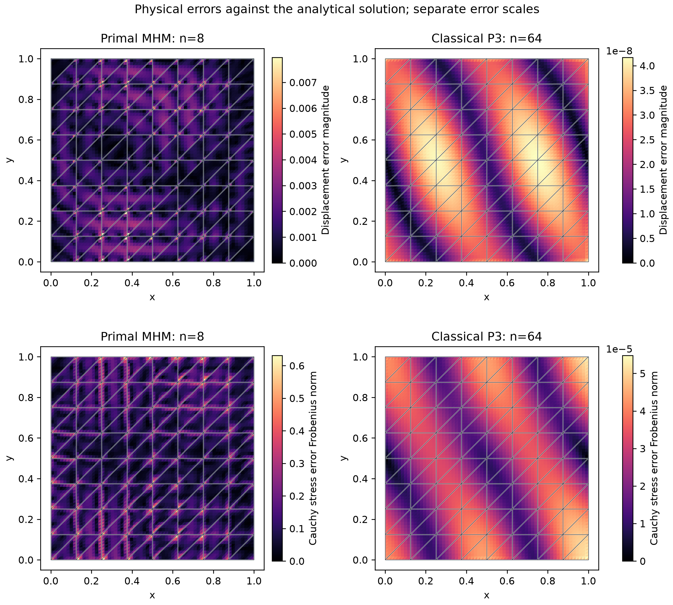
The classical reference itself refines at orders 4.0057 and 4.0026 for displacement, and 2.9997 and 3.0000 for stress. These are its conforming P3 rates, not the P1-traction MHM rates. On the finest classical grid, its displacement error is below 1% of the finest MHM error and its stress error below 1.9%. Original free-equilibrium relative residuals remain below \(7.6\times10^{-12}\); the largest relative change under independent norm quadrature refinement is \(4.91\times10^{-9}\). The exact solution remains the source of the convergence errors; the classical solution is a checked numerical baseline.

Matched classical refinement record

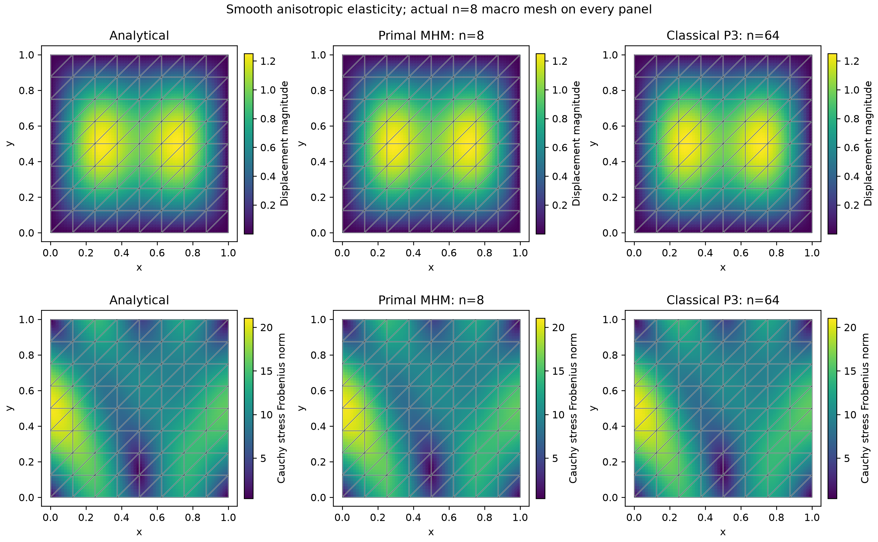
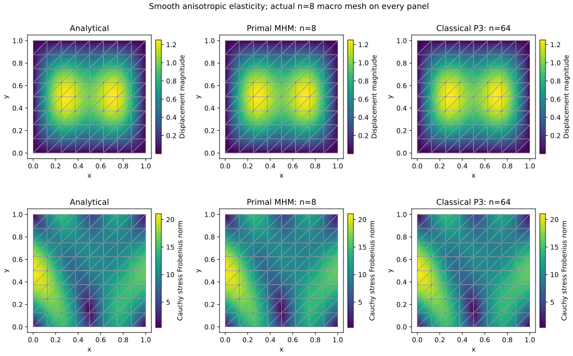
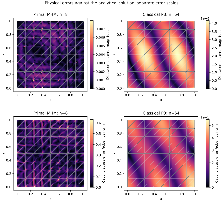
The panels below use the first measured MHM grid, \(n=8\), and the conforming P3 grid \(n=64\). The MHM keeps one local triangle per macrocell and its P1 traction space; the classical reference solves on its independent finer global mesh. Every panel highlights the actual \(n=8\) macro mesh. Physical fields share their color scales, while error panels use separate scales with their actual values. Independent incident reconstructions preserve macroface discontinuities.

Field SVG · Field PDF

Error SVG · Error PDF · Field acquisition record

References

• Christopher Harder, Alexandre L. Madureira, and Frédéric Valentin (2016). A hybrid-mixed method for elasticity, ESAIM: M2AN 50, 311–336. DOI: 10.1051/m2an/2015046.