Direct field comparison with MSL
This case compares complete numerical fields from pyMHM and the IPES/LNCC
MSL implementation: msl_mhm for MHM coupling, msl_cg for continuous
Galerkin local problems, and msl_core for shared infrastructure. Both primal
MHM solvers solve the same problem with the same macro mesh, local
finite elements, skeleton space, and boundary enforcement. Across five mesh
sizes, full-field L2 differences stay below \(5.1\times10^{-14}\) in pressure and
\(4.5\times10^{-13}\) in flux. The largest case contains 65,536 fine triangles.
The coarse cosine comparison separately checks the gallery's diagonal mesh and P0 traces. Both comparisons use the same boundary assembly; their prescribed pressures are zero and nonzero, respectively.
Reference code and revisions
The label MSL in the figures refers to the following combination, using the
main_mhm_diffusion example from msl_mhm:
| Component | Role | Executed revision |
|---|---|---|
ipes-lncc/msl_mhm |
MHM local/global coupling and diffusion driver | 4cb8cf81518284313b680b13fd586ee619f08b99 |
ipes-lncc/msl_cg |
DiffusionCGProblem local finite element assembly |
afb76d14c1baf50f0b9e69f7bcac675749ef4458 |
ipes-lncc/msl_core |
Mesh, approximation-space and algebra infrastructure | 7f15f455717173d29080d411a7e732c72c1e87f8 |
The executable instantiates
MHMGlobalProblem<DiffusionCGProblem, CGMHMDecorator<DiffusionCGProblem>>.
MSL's numerical libraries and solve sequence are unchanged. The comparison
adapter assembles prescribed weak Dirichlet boundary moments and exports fields
and error norms at 17-digit precision. The archived report records the component
revisions and the adapter's source digests.
Problem and identical discretization
On \(\Omega=(0,1)^2\),
with exact pressure \(p=\sin(2\pi x)\sin(2\pi y)\) and physical flux \(\boldsymbol q=-\nabla p\).
Each Cartesian macro square is divided into four triangles through its center. The partitions have 4, 16, 64, 256, and 1024 macrotriangles. Within every macrotriangle, each edge is divided into eight equal segments, producing 64 fine triangles and 45 continuous P1 pressure unknowns. The skeleton is P1 on each unsplit macro edge. Thus \(h=H/8\) throughout the sequence.
Dirichlet pressure is imposed weakly through the global skeleton moments. Every local solve is a Neumann problem with a constant kernel and its physical mean constraint. This choice matters: strong nodal Dirichlet constraints on boundary macroelements produce a different finite dimensional method and cannot serve as an identical-discretization comparison.
MSL uses C++ finite element assembly and Eigen sparse LU. Its export records pressure coefficients, triangle connectivity, and error norms. PyMHM uses its NumPy/SciPy implementation. Both use accurate forcing and error quadrature; PyMHM uses Gauss-Duffy order 8, while MSL's forcing parameter 8 requests native polynomial integration degree 9. These are different rules, despite the same input integer. Reintegrating the exported MSL fields with PyMHM's quadrature recovers MSL's computed errors to rounding accuracy.
Results against the analytic solution
| Macrotriangles | \(H\) | MSL pressure \(L^2\) | PyMHM pressure \(L^2\) | MSL raw flux \(L^2\) | PyMHM raw flux \(L^2\) |
|---|---|---|---|---|---|
| 4 | 1 | 1.42098571e-01 | 1.42098571e-01 | 2.10096391e+00 | 2.10096391e+00 |
| 16 | 0.5 | 1.16904455e-01 | 1.16904455e-01 | 1.81630493e+00 | 1.81630493e+00 |
| 64 | 0.25 | 6.88512796e-03 | 6.88512796e-03 | 3.43688530e-01 | 3.43688530e-01 |
| 256 | 0.125 | 9.10320678e-04 | 9.10320678e-04 | 1.38270851e-01 | 1.38270851e-01 |
| 1024 | 0.0625 | 1.51680908e-04 | 1.51680908e-04 | 6.42761266e-02 | 6.42761266e-02 |
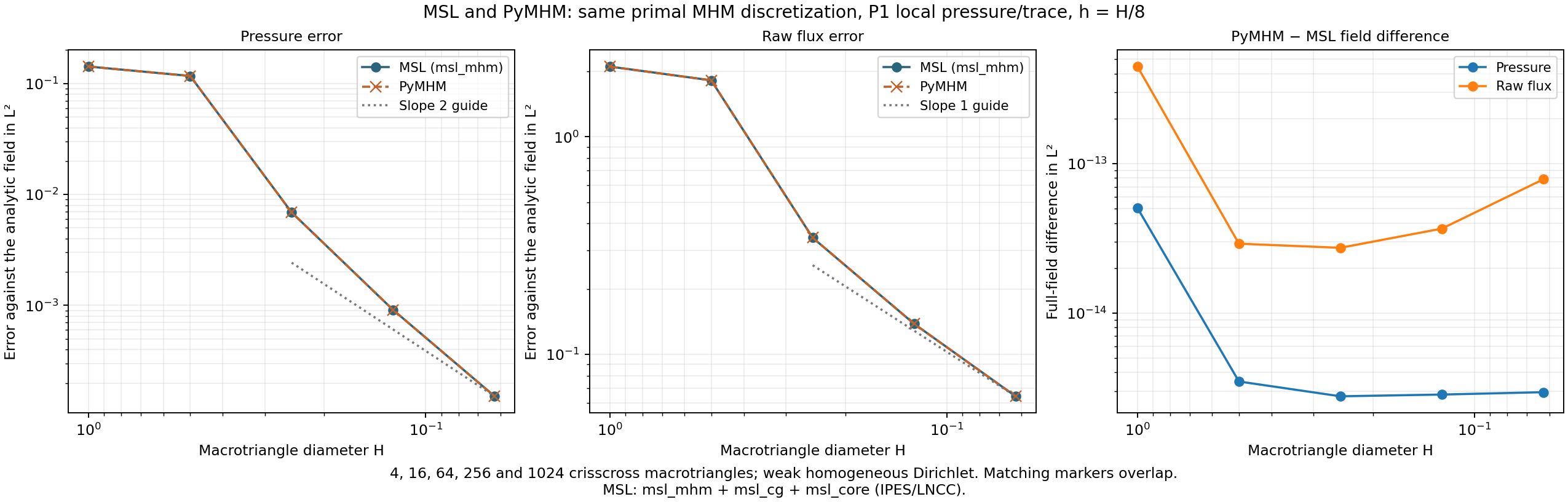
The first two coarse meshes underresolve the oscillatory solution. Asymptotic behavior should be assessed on the finer meshes, rather than inferred from those two points. The slope guides are references, not fitted convergence claims. The raw primal flux is the piecewise constant field \(-\nabla p_h\); this experiment does not replace it with an equilibrated \(H(\mathrm{div})\) reconstruction.
Agreement of the full fields
Matching each local node by its physical coordinate, and each fine triangle by its three vertex coordinates, avoids assumptions about either code's numbering and orientation. Pressure differences are integrated exactly using the P1 mass matrix; raw flux differences are integrated exactly as P0 fields. Across the five meshes:
- pressure field differences in \(L^2\) are at most \(5.05\times10^{-14}\);
- raw flux field differences in \(L^2\) are at most \(4.47\times10^{-13}\);
- the largest nodal pressure difference is \(1.04\times10^{-13}\);
- the largest raw flux component difference is \(1.42\times10^{-12}\).
These measurements use the recorded coefficient-by-coefficient comparison, rather than inferring agreement from overlapping error curves. The retained JSON includes the checksums of the original field snapshots; those coefficient snapshots are not distributed with this checkout. Consequently, this page shows the retained norms and full-field differences, and does not present a spatial MSL reconstruction from unavailable coefficients.
Inspect the archived results
The full precision numerical report retains the five mesh levels, component revisions, comparison metrics and SHA-256 checksums. MSL source and comparison execution programs are not distributed. The convergence figure can be regenerated from this report without an MSL installation or another finite element solve:
import json
from pathlib import Path
from examples.plot_reference_comparison import plot_errors

report = json.loads(
    Path("examples/results/reference-darcy-comparison.json").read_text()
)
plot_errors(report)
The executed verification checked every pressure coefficient and every raw flux
component against the MSL solution. Its tolerances allow platform-dependent
floating point roundoff and are much smaller than the discretization errors.
The plotter displays those measurements; it does not rerun the verification.
The original reference-darcy-*.npz and aligned field snapshots are required
to replay spatial reference fields. New PyMHM solves cannot replace those
snapshots while retaining their original acquisition checksums. The
coarse cosine report includes a
separate, downloadable physical-field replay against native NeoPZ evaluation.
Relation to the literature and other backends
The sine problem is also used in the unfitted flux study discussed in Chaumont-Frelet, Paredes and Valentin (2026). That article fixes 16 macrotriangles and refines the skeleton, with local problems solved to sufficient accuracy. This experiment instead refines both macro and local meshes with fixed local ratio and P1 local approximation. It verifies agreement between MSL and pyMHM; it does not claim to reproduce that article's convergence curve or a P2/RT2 reconstruction table. The Darcy gallery separately distinguishes raw and conservative flux approximations.
An additional run of ipes-lncc/msl_mfem, revision
b9a67e7079c7e487e4ab1679c1bb3c880cc1909a, using MFEM 4.9 and
strong local Dirichlet conditions,
produced pressure error approximately \(2.81519\times10^{-2}\) on four
macrotriangles. The msl_mhm + msl_cg strong-boundary counterpart gave
\(2.81496\times10^{-2}\), while the weak-boundary method above gives
\(1.42099\times10^{-1}\). These numbers belong to different discrete boundary
conditions and integration rules, so they are not used as a PyMHM agreement
claim. This page's matched weak-boundary comparison uses msl_mhm + msl_cg.
The software provenance distinguishes
these components from the separate ipes-lncc/mhm-mfem project.
References
- Théophile Chaumont-Frelet, Diego Paredes, and Frédéric Valentin (2026). Flux approximation on unfitted meshes and application to multiscale hybrid-mixed methods, Computers & Mathematics with Applications 209, 16–27. DOI: 10.1016/j.camwa.2026.01.016.