Three-dimensional Darcy: native workspaces, LU and AMG

The introductory notebook defines the material, manufactured fields, local UFL forms, oriented trace pairings, global equations, reference methods and physical norm integration in executable cells. It introduces reusable native assembly resources after showing the mathematical forms. A small default demonstration accompanies the recorded 3D campaign.

The CPU PARDISO and GPU extension reports larger local grids, CPU strong/weak scaling and one/two-GPU complete workflows. Its acquisitions and field controls have separate immutable provenance.

Physical problem and two material periods

On the box with integer length,

\[ \Omega_L=(0,L)\times(0,1)^2, \]

solve

\[ \begin{aligned} q&=-K\nabla p, & \nabla\cdot q&=f,\\ p&=0 &&\text{on }\partial\Omega_L. \end{aligned} \]

The manufactured fields and material are

\[ \begin{aligned} p_*(x)&=\prod_{i=1}^3\sin(\pi x_i),\\ K(x)&=m_\varepsilon(x)D, & m_\varepsilon(x)&=\exp\!\left(\prod_{i=1}^3\sin(2\pi x_i/\varepsilon)\right),\\ D&=\begin{pmatrix}2&0.3&0.2\\0.3&1.5&0.1\\0.2&0.1&1\end{pmatrix}, & f&=\nabla\cdot(-K\nabla p_*). \end{aligned} \]

The tensor is symmetric positive definite. Its off-diagonal entries require mixed pressure derivatives in the source. UFL differentiation and independently derived analytical formulas specify the same physical operator and source. Integer domain lengths preserve the exterior pressure data; the coefficient wavelength remains fixed when the box expands.

Here ε is the permeability spatial period, measured in coordinate units. The principal material period is 0.1 and the macro width is 0.25. The scalar multiplier consequently equals one on every macroface, where its coordinate factors contain sine values at integer multiples of five pi. This alignment is a feature of these data and affects skeleton approximation. A separate period-0.137 case removes that alignment. Its 64 material matrices are all distinct; its timings and errors are reported separately. Neither material case reuses numerical factors or local responses between macrocells.

Local and global discretization

The unit cube has 64 macrohexahedra. Each contains a structured conforming Q1 local volume mesh. Fine counts of 64 or 96 per unit direction give 16 or 24 local cells per direction, hence 262,144 or 884,736 total fine hexahedra. The independent conforming reference uses the same fine grid. The optional 128-per-direction configuration is not a completed measurement in this record.

Each unsplit macroface carries four tensor-product Q1 modes. The unit-cube skeleton has 240 faces, 960 trace coordinates and 64 retained constants; the coupled system has 1,024 coordinates. These spaces differ from the conforming reference's global Q1 space. The local equations are

\[ \begin{aligned} a_T(p_T,v)+b_T(v,\lambda)&=(f,v)_T,\\ a_T(p,v)&=\int_T K\nabla p\cdot\nabla v,\\ b_T(v,\lambda)&=\sum_{F\subset\partial T}s_{T,F}\int_F v\lambda_F. \end{aligned} \]

The sign maps the canonical face flux into each cell's outward orientation. Increasing physical tangent coordinates define the same face basis on both sides in this Cartesian application. Basix tabulates field and trace bases; DOLFINx/UFL assembles the declared volume and face forms.

The local kernel is the constant function. Physical volume moments select zero-mean source and trace responses; the retained constant restores the physical cell mean. Full Dirichlet pressure data impose no global zero-mean gauge: the exact unit-cube mean is nonzero. The global coupling tests pressure continuity with the pairing c=-b.T and retains the constant compatibility rows. LocalEquations, Equation and MultiscaleProblem perform condensation, assembly and reconstruction without a physical-model constructor.

The Darcy flux evaluated here is the broken field -K grad(p_h). It is not an H(div) reconstruction. Macro conservation of oriented trace moments does not imply pointwise interface continuity or fine-cell conservation. Field plots overlay the actual macro mesh and retain independent one-sided values.

Reuse native resources without reusing material solves

A process or concurrent thread owns its native workspace. The cache key includes volume and trace degrees, local topology/resolution, quadrature, physical cell extents and dtype. Compatible calls reuse the local mesh, finite element spaces, compiled UFL kernels and assembly buffers. Pickle transfers only declarations, and the executor closes native resources after running work completes. Incompatible keys build another bounded workspace.

For every macrocell, the application updates physical geometry and the material's declared UFL constants, then assembles a fresh material matrix and source. Returned arrays own their data. Each material matrix gets its own factorization or AMG hierarchy and source/trace solves. No material parity, periodicity or response basis is used as a cache key.

Only unsigned trace and volume-moment blocks are reused here: their UFL forms contain geometry but no material coefficient. Face signs and global indices are applied anew for each macrocell. This application-specific independence must be rechecked for Robin or material-weighted coupling forms; the generic backend makes no such assumption.

Independent native controls compare fresh and reused matrices, loads, oriented couplings, kernels, physical moments, retained bases, source/trace responses and full reconstructed fields. They include a material change and return, nonaligned coefficients, concurrent threads and spawned processes. The record preserves original physical equations and executed basis digests, so replay does not recompute an arbitrarily oriented nullspace.

Solvers and measured timing scope

Direct local solves use SciPy SuperLU or PETSc/MUMPS on MPI.COMM_SELF. A factorization serves the source and 24 trace right-hand sides of one macrocell; it is rebuilt for another material matrix. CPU PyAMG uses the shared Neumann projection, coordinate pinning and physical-moment restoration owner. Its original-row refinement stays inside that owner and timer. A hierarchy serves multiple right-hand sides within a solver call; additional refinement passes can rebuild a hierarchy. The coupled global problem retains sparse direct algebra rather than an elliptic AMG preset.

The independent classical comparison uses distributed PETSc/MUMPS LU or PETSc CG/GAMG on the same grid, material, source and full Dirichlet data. Thirty-two physical cores are available to the large parallel configurations, with one native thread per process or MPI rank. A serial classical large-grid LU measurement is not present. Classical GAMG and local PyAMG are different AMG implementations and solve different global algebraic structures.

Reported complete times start at the parent launch and include interpreter imports, native initialization, geometry and forms, fresh material assembly, solver setup, response transfers, synchronization, shared-face accumulation, worker shutdown, global solution and reconstruction. Error integration, archive writing and plotting occur afterward. Compiler warmup populates the existing cache; measurements include fresh workers but exclude cold FFCx/JIT compilation. Raw records also retain the solver-pipeline time and startup cost separately. Per-process RSS high-water marks do not establish a simultaneous aggregate memory peak.

Each accepted configuration is an actual completed sample. Timing windows separate competing project workloads. The measurements do not establish statistical variance, multi-node scaling or a large GPU speedup. The optional one-/two-GPU local-condensation procedure has a separate timing scope; no accepted large GPU timing is available in this edition.

Strong scaling

Strong scaling fixes the full period-0.1 unit-cube discretization: 262,144 fine cells, 64 macrocells, Q1 volume/face spaces and 1,024 coupled coordinates. Each MHM curve uses one spawned process as its denominator, with fresh imports and worker setup. MHM configurations expose the same 32 physical cores with one native thread per worker. The classical CG/GAMG curve uses its own one-MPI- rank denominator and assigns one physical core per rank. Actual process/rank counts are 1, 2, 4, 8, 16 and 32. A serial call without a spawned worker is a different timing configuration.

Local solver	Processes	Complete launch time (s)	Self-speedup	Efficiency (%)
MHM MUMPS LU	1	41.4881	1.000	100.00
MHM MUMPS LU	2	23.8736	1.738	86.89
MHM MUMPS LU	4	14.3390	2.893	72.33
MHM MUMPS LU	8	8.7468	4.743	59.29
MHM MUMPS LU	16	6.1865	6.706	41.91
MHM MUMPS LU	32	5.1665	8.030	25.09
MHM PyAMG	1	109.5554	1.000	100.00
MHM PyAMG	2	58.0224	1.888	94.41
MHM PyAMG	4	31.3542	3.494	87.35
MHM PyAMG	8	18.7695	5.837	72.96
MHM PyAMG	16	11.7759	9.303	58.15
MHM PyAMG	32	8.2986	13.202	41.26

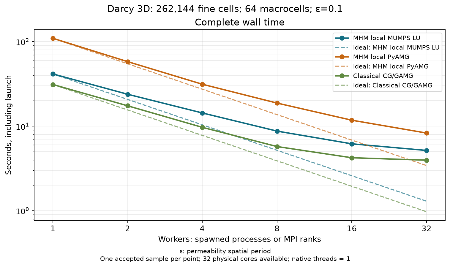
Complete measured wall time and ideal T(1)/P references; markers identify acquired configurations.

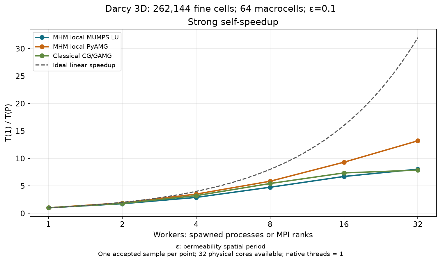
Strong process self-speedup, with the ideal linear reference.

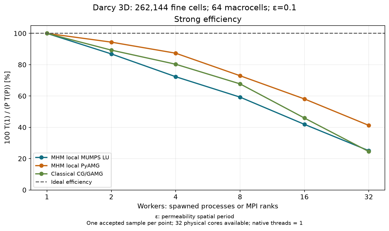
Strong efficiency S(P)/P: startup, transfers and global work remain in the total.

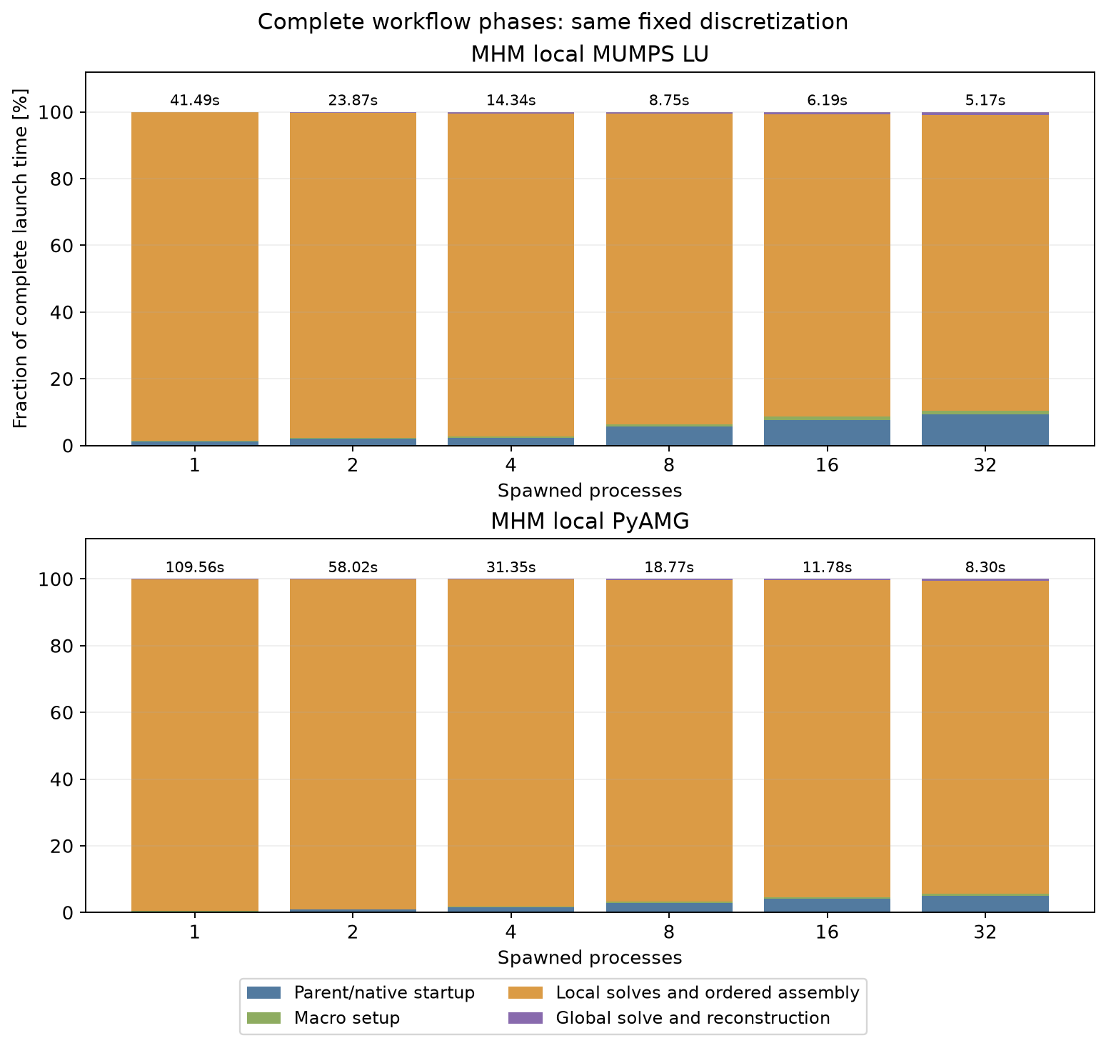
Complete workflow phase fractions and actual elapsed seconds; local/ordered assembly includes independent material solves and worker communication.

Focused weak scaling

Within each curve, macro width is 0.25, fine-cell width is 1/64, the material period and trace degree stay fixed, and both fine and macro cells per process are constant. The x-domain expands through integer lengths. Four- and eight-macrocell-per-process families remain separate. The baseline is the smallest actually measured process count in that family, not an assumed one-process run. Efficiency is its complete time divided by the measured larger-domain time. Growth of the skeleton and global solve remains included. These short curves establish focused node-local observations, rather than asymptotic or multi-node weak scalability.

Permeability spatial period, ε	Local solver	Macrocells / process	Processes	Box length	Fine cells	Coupled coordinates	Complete launch time (s)	Weak efficiency (%)
0.1	MHM MUMPS LU	8	8	1	262,144	1,024	8.7468	100.00
0.1	MHM MUMPS LU	8	16	2	524,288	1,984	14.4457	60.55
0.1	MHM MUMPS LU	8	32	4	1,048,576	3,904	18.7764	46.58
0.1	MHM PyAMG	4	16	1	262,144	1,024	11.7759	100.00
0.1	MHM PyAMG	4	32	2	524,288	1,984	20.0016	58.87
0.1	MHM PyAMG	8	8	1	262,144	1,024	18.7695	100.00
0.1	MHM PyAMG	8	16	2	524,288	1,984	24.3604	77.05
0.1	MHM PyAMG	8	32	4	1,048,576	3,904	29.7701	63.05
0.137	MHM MUMPS LU	4	16	1	262,144	1,024	6.3699	100.00
0.137	MHM MUMPS LU	4	32	2	524,288	1,984	13.5564	46.99

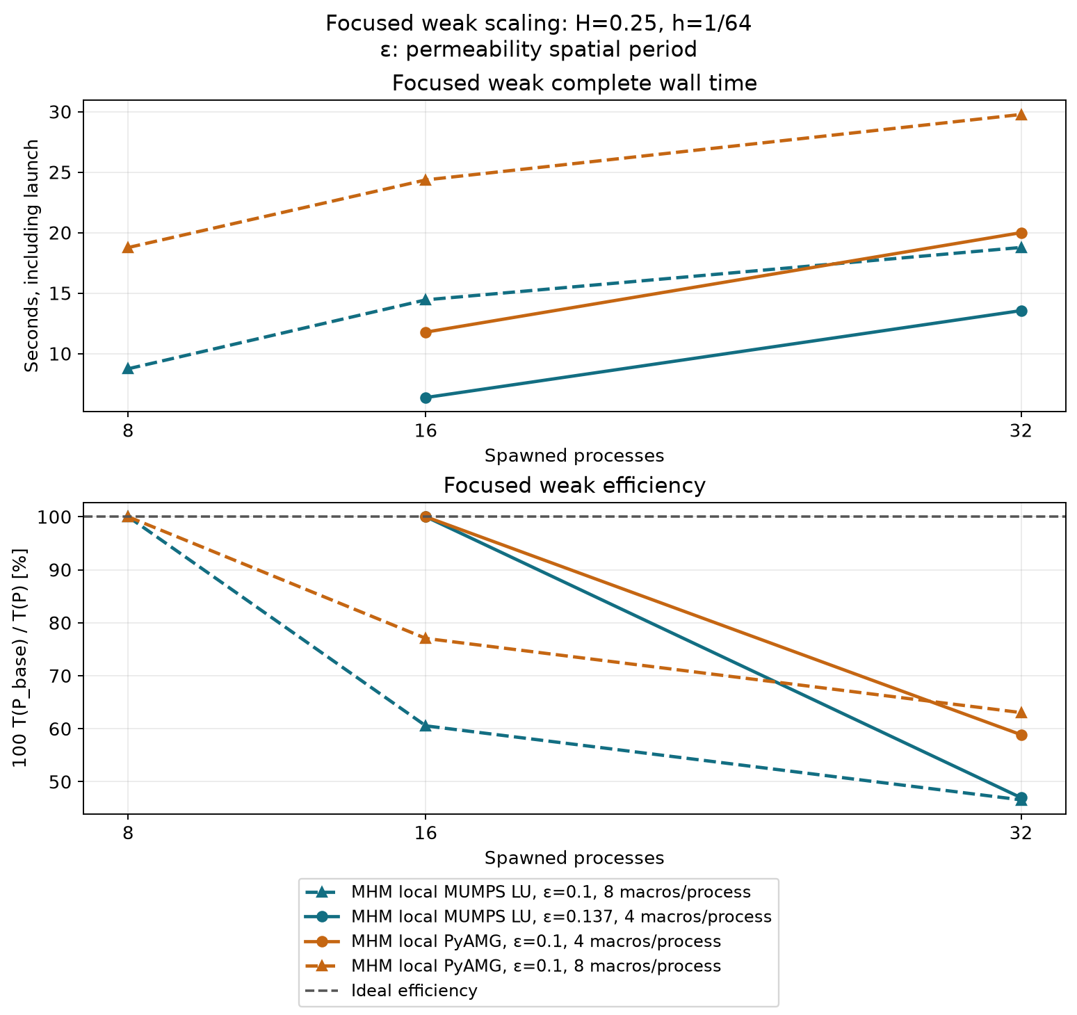
Focused weak complete wall time and efficiency; each legend identifies its fixed work per process.

Cost and physical accuracy

Permeability spatial period, ε	Fine cells per unit axis	Method	Processes / ranks	Complete launch time (s)
0.1	64	Classical PETSc CG/GAMG	32	3.9623
0.1	64	Classical PETSc PREONLY/LU/MUMPS	32	16.8697
0.1	64	MHM MUMPS LU	32	5.1665
0.1	64	MHM PyAMG	32	8.2986
0.1	64	MHM SuperLU	32	6.0051
0.137	64	Classical PETSc CG/GAMG	32	3.7496
0.137	64	Classical PETSc PREONLY/LU/MUMPS	32	16.6027
0.137	64	MHM MUMPS LU	32	5.0159
0.137	64	MHM PyAMG	32	7.9710
0.1	96	Classical PETSc CG/GAMG	32	9.2592
0.1	96	Classical PETSc PREONLY/LU/MUMPS	32	96.3061
0.1	96	MHM MUMPS LU	32	10.4146
0.1	96	MHM PyAMG	32	22.5916
0.1	96	MHM SuperLU	32	56.0215

At matched 32-physical-core and fine-element budgets, local MUMPS MHM is 3.27× faster than classical distributed MUMPS at 64 cells per unit axis and 9.25× faster at 96. The period-0.137 LU comparison gives 3.31×. These are measured workflow ratios for different approximation spaces, with the physical errors shown alongside them. They are not equal-accuracy speedups.

Classical distributed CG/GAMG remains faster than both MHM local MUMPS and MHM local PyAMG at the measured unit-cube resolutions. The favorable LU comparison therefore does not establish an advantage over the best classical solver measured here. Each timing point is an actual completed sample; no confidence interval or variance estimate is inferred.

Permeability spatial period, ε	Fine cells per unit axis	Approximation	Pressure L2 error	Physical vector-flux L2 error
0.1	64	Conforming Q1	8.8900421e-05	4.8283419e-02
0.1	64	MHM; macro4 / traceQ1	1.0714369e-03	7.5135753e-02
0.137	64	Conforming Q1	8.9063230e-05	4.8612283e-02
0.137	64	MHM; macro4 / traceQ1	5.8898023e-03	4.1392472e-01
0.1	96	Conforming Q1	3.9629110e-05	3.2451356e-02
0.1	96	MHM; macro4 / traceQ1	1.0801716e-03	6.6169010e-02

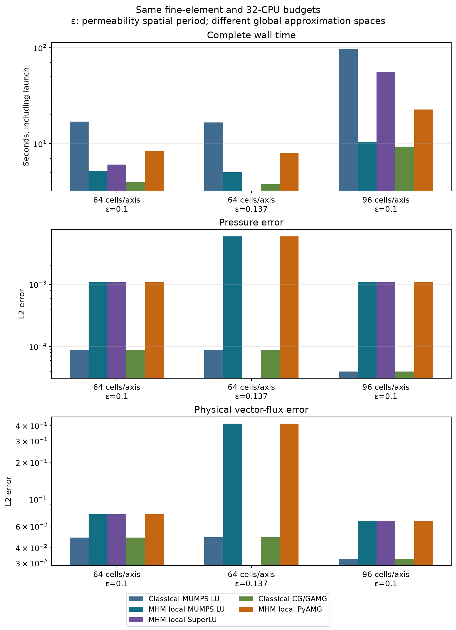
Fine-element and 32-CPU budget comparisons display time, pressure error and physical vector-flux error together. Approximation spaces differ. Empty solver slots are unmeasured configurations; absent field integrals are labeled explicitly.

Pressure and vector-flux errors are integrated separately against the exact fields. Refining only local volume meshes with a fixed macro grid and Q1 trace leaves a pressure-error floor: the period-0.1 MHM pressure error stays near 1.08e-3 while the flux error decreases. This is a local-resolution performance sweep, not complete MHM convergence. The nonaligned period changes both volume and face permeability and gives larger MHM field errors in the same fixed trace space. Its interface-resolution study is a separate experiment; the aligned case's accuracy is not transferred to these data. The conforming method's own refinement and quadrature controls remain independent of the performance ratios.

Literature and scope

Gomes et al. (2017, preprint v1) separate independent local response construction from the coupled global solve, with MPI ownership and distributed algebra. Their published 3D experiment has different coefficients, tetrahedral P2 spaces, face partitions and cluster resources. This Q1 hexahedral analytical application is not a reproduction of that timing table; the simplex error estimates are not asserted for these cube spaces.

Penna et al. (2019) investigate cost-aware scheduling for heterogeneous MHM work. Their measured gains do not transfer to uniform local meshes without a matching experiment. The present curves use bounded node-local process execution, and establish no multi-node or large GPU gain. The execution guide specifies resource ownership and cleanup.

References

• Antônio Tadeu A. Gomes, Weslley S. Pereira, Frédéric Valentin, and Diego Paredes (2017). On the Implementation of a Scalable Simulator for Multiscale Hybrid-Mixed Methods, arXiv preprint, version 1, 30 March 2017. arXiv: 1703.10435v1.

• Pedro Henrique Penna, Antônio Tadeu A. Gomes, Márcio Castro, Patricia D.M. Plentz, Henrique C. Freitas, François Broquedis, and Jean‐François Méhaut (2019). A comprehensive performance evaluation of the BinLPT workload‐aware loop scheduler. Concurrency and Computation: Practice and Experience 31(18) e5170. DOI: 10.1002/cpe.5170.