Three-dimensional Darcy: CPU direct solvers and GPU local solves

The introductory notebook defines the manufactured Darcy problem and the local/global mathematical forms. This performance study extends that application with CPU PARDISO and independent GPU local solves. The immutable accelerator edition contains the selected raw acquisitions, their own numerical controls and the plotted summaries. The earlier workspace/LU/AMG edition retains its original results; its CPU weak observations appear as separately identified historical references here.

Physical problem and fixed approximation spaces

The physical formulation specifies the anisotropic multiscale permeability, independent manufactured source, exact pressure/flux and full exterior pressure boundary data. Here ε means the permeability spatial period in physical coordinates. Every timed case in this edition uses ε=0.1. It is fixed when the domain grows; it is not a solver tolerance or a viscosity parameter.

The domain family is

\[ \Omega_L=(0,L)\times(0,1)^2,\qquad L\in\mathbb{N}. \]

Macro width remains 0.25. A resolution parameter n gives n fine hexahedra per unit direction and n/4 local cells per macro direction. Total fine cells are Ln³, with 64L macroelements. Local pressures use Q1; each unsplit macroface has four tensor-product Q1 trace modes. Neither the macro mesh nor the trace degree changes in the larger local-grid experiments.

The classical conforming reference uses the same physical operator, material, boundary data and fine Q1 grid. Its global conforming space differs from the MHM space. Equal fine-element counts and CPU budgets therefore establish a workload comparison, not equal pressure/flux accuracy. The fixed macro/trace spaces can produce a pressure-error floor as local meshes refine.

The physical Dirichlet pressure gauge is preserved. There is no global zero-mean constraint: the exact mean is (2/π)³ for L=1, (2/π)³/3 for L=3, and zero for L=2 or 4. Local source/trace responses have zero physical volume moment; the retained constant restores the local physical mean. The reported Darcy flux is the broken physical field −K∇p_h, with no H(div) or fine-cell conservation claim.

CPU and GPU workflows

Classical PARDISO uses native FEM assembly on MPI.COMM_SELF, followed by a sparse PARDISO factorization with 32 suggested MKL threads. MHM PARDISO uses independent spawned CPU workers, with one MKL thread per worker. The direct factor profile is general LU, PARDISO mtype11; a local constrained Neumann system is indefinite and is not assigned an SPD factor profile. A factor serves all right-hand sides for its own macroelement and is rebuilt for another material matrix.

The classical acquisition permits 32 native threads throughout its setup, assembly and solve block; the factorization receipts observe a MKL32 thread-pool limit. Native FEM assembly on COMM_SELF is serial, with no MPI decomposition. The introductory native call that limits threads only around factorization has its own resource scope. Observed native pool limits describe available capacity, rather than measuring the number of threads participating in every operation.

These resource conventions distinguish parallel factorization from distributed FEM assembly. The earlier classical PETSc/GAMG and PETSc/MUMPS references use MPI distributed assembly; local PyAMG and classical GAMG are different AMG implementations. Raw receipts preserve the actual native environments, library versions and observed thread settings. Cross-workflow timing differences do not isolate a solver-library or accelerator effect.

For the GPU workflow, CPU workers first assemble the local UFL operators with resident native workspaces. Independent GPU-owning processes then receive their assigned operators, create fresh factors or AMG hierarchies and solve the source and trace right-hand sides. Each process owns its native CUDA context and device resources. Returned responses enter ordered global assembly, the global solve and reconstruction through the same generic MHM interfaces.

Compatible native meshes, spaces, compiled forms and geometry-only blocks are reused inside each worker. Material matrices and loads are assembled for each macroelement. No numerical factor, hierarchy or response is reused across different material matrices or acquisitions. The GPU-process stage is a phase of this complete workflow, not a component measurement added to a separately measured CPU median.

Complete clocks and numerical acceptance

The edition contains 40 new acquisitions: 32 MHM states and eight classical references. Each has its own integrated pressure and physical vector-flux norms. Six historical CPU weak samples retain their original controls; one has its own integrated norms and five retain null norms. They are separate observations from the earlier edition.

The complete clock starts at the external parent launch. It includes interpreter imports, native initialization, application setup, material assembly, CPU/GPU pool creation and shutdown, scheduling/serialization, transfers, matrix analysis and factor/hierarchy setup, all right-hand sides and residual corrections, device synchronization, ordered global work and field reconstruction. Form compilation is warmed separately; workers, material matrices and factors remain fresh in every timed acquisition. Archive writing, physical error integration and plotting follow the competitive clock.

Every accepted MHM acquisition records its original local operators, source/trace responses, executed retained basis, coefficient vectors, orientations and reconstructed physical fields. SHA-256 binds the whole state and each executed retained basis. Its own post-timing control replays the field with BLAS one/two threads and equivalent rank-one basis sign rotations, including the trace orientation map. Physical volume moments, original kernel action and each source/trace/reconstructed physical row have separate recorded controls. Source/trace responses and the reconstructed original physical equations satisfy the declared 1e−10 relative residual gate. The kernel action is measured at operator scale, and declared physical volume moments retain their own absolute discrepancies. The relative diagnostic for the retained action AZ uses a right-hand side at roundoff scale; its small denominator can produce a sizable ratio, which is recorded separately from the physical-row acceptance gate. The executed retained basis remains part of the archived coefficient contract. The coupled residual has a separate recorded gate.

Classical archives contain the actual physical Q1 nodal coefficients and their integer-lattice coordinate convention. Native UFL replay integrates those unchanged coefficients collectively. Their assembled-matrix residual belongs to the acquisition; a field-only replay does not recompute an unpersisted matrix.

Pressure and physical vector-flux errors are integrated separately from these algebraic checks. Each marker belongs to the same timed acquisition's own field. MHM Gauss5→6 and native classical quadrature degree10→12 control pressure and flux norm changes separately; higher orders are used when the relative change exceeds 1e−6. A state without error integration retains null norms, with explicit provenance. No error norm is copied from another state or repetition.

For expanding domains, the record retains both absolute errors and

\[ \begin{aligned} e_p&=\frac{\lVert p_h-p_*\rVert_{L^2(\Omega_L)}} {\sqrt{\lvert\Omega_L\rvert}},\\ e_q&=\frac{\lVert q_h-q_*\rVert_{L^2(\Omega_L)}} {\sqrt{\lvert\Omega_L\rvert}}. \end{aligned} \]

Configuration summaries use arithmetic means of the actual selected repetitions. Whiskers give observed extrema; they are not confidence intervals. Each source/lockfile digest, resource allocation, native version, parameter set and timing scope remains bound to its original raw acquisition.

CPU strong scaling

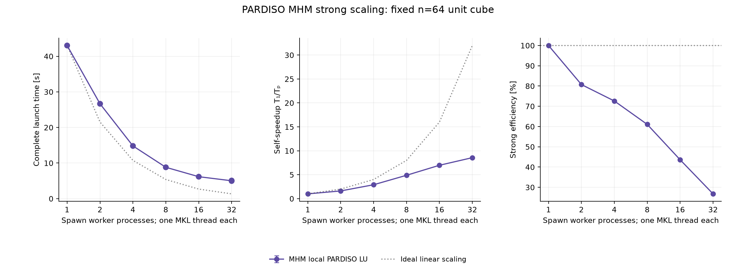
The PARDISO strong family fixes the n=64 unit-cube discretization and varies spawned workers through 1, 2, 4, 8, 16 and 32, with one MKL thread per worker. Its denominator is the measured one-spawn-process complete launch. The wall-time, self-speedup and efficiency panels include their corresponding ideal references.

Workers	Complete time [s]	Self-speedup	Efficiency [%]	Samples
1	43.03	1.00	100.0	1
2	26.65	1.61	80.7	1
4	14.81	2.90	72.6	1
8	8.81	4.88	61.1	1
16	6.17	6.97	43.6	1
32	5.02 [4.96, 5.09]	8.57	26.8	2

At 32 workers the observed PARDISO self-speedup is 8.57×, with 26.8% strong efficiency. The same-grid direct comparisons use the complete workflows and resource conventions above:

n	Fine hexahedra	Classical PARDISO [s]	MHM PARDISO [s]	Classical/MHM time
64	262,144	27.05 [26.94, 27.15]	5.02 [4.96, 5.09]	5.38
96	884,736	109.15 [108.90, 109.41]	9.99 [9.96, 10.03]	10.92
128	2,097,152	351.07	21.57	16.28

These ratios compare decomposition and assembly as well as factorization. The approximation spaces and physical errors differ; they are not gains at equal accuracy. Brackets give observed extrema of two actual repetitions.

CPU weak scaling

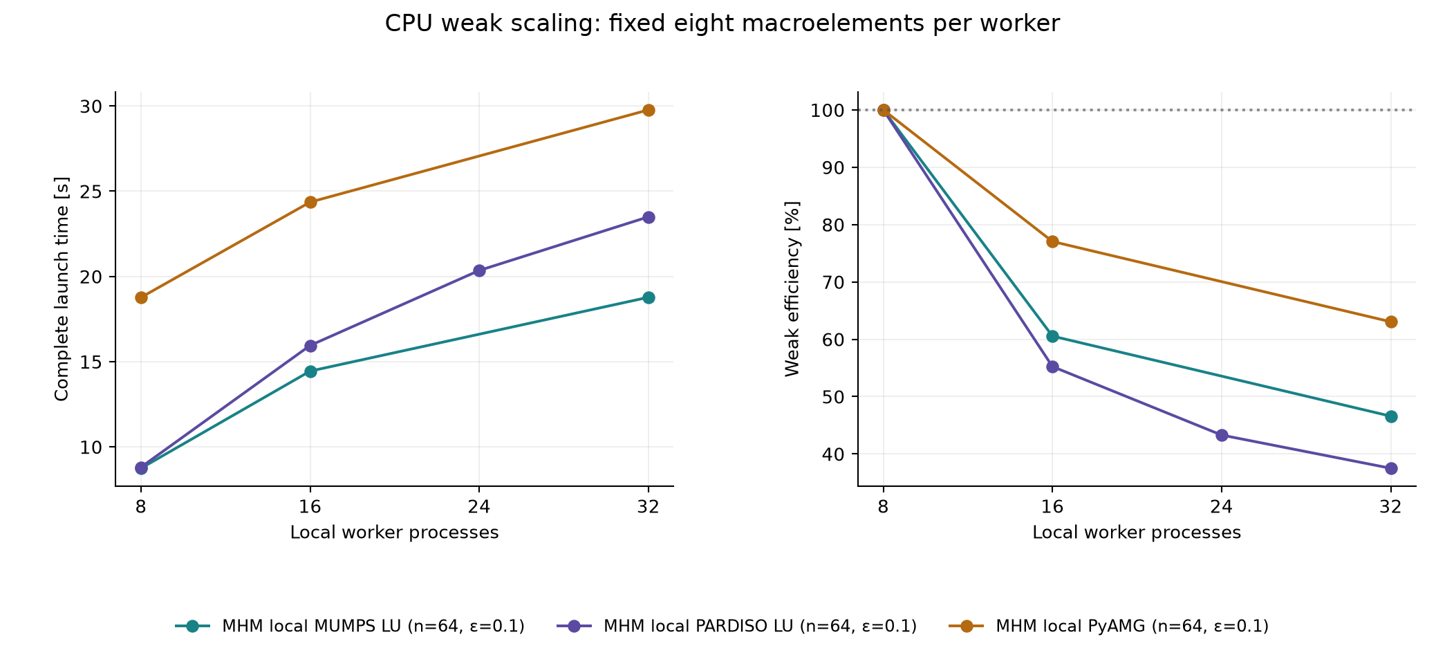
The CPU family retains eight macroelements per worker, fixed local resolution and fixed permeability spatial period. Worker counts 8, 16, 24 and 32 use integer domain lengths 1, 2, 3 and 4 for PARDISO; historical MUMPS/PyAMG references retain their actual 8, 16 and 32 acquisitions. Weak efficiency is

\[ \eta_{\mathrm{weak}}(P)=\frac{T(P_0)}{T(P)}. \]

There is no extra factor P/P₀. Growing global work and communication remain in the complete time. Historical curves preserve their separate source/resource provenance and their measured efficiency losses.

Local solver	Workers	L	Complete time [s]	Weak efficiency [%]	\(e_p\)	\(e_q\)
PARDISO	8	1	8.81	100.0	1.0714e-03	7.5136e-02
PARDISO	16	2	15.95	55.2	1.0716e-03	7.5143e-02
PARDISO	24	3	20.35	43.3	1.0717e-03	7.5145e-02
PARDISO	32	4	23.50	37.5	1.0717e-03	7.5146e-02
MUMPS (historical)	8	1	8.75	100.0	—	—
MUMPS (historical)	16	2	14.45	60.5	—	—
MUMPS (historical)	32	4	18.78	46.6	1.0717e-03	7.5146e-02
PyAMG (historical)	8	1	18.77	100.0	—	—
PyAMG (historical)	16	2	24.36	77.0	—	—
PyAMG (historical)	32	4	29.77	63.0	—	—

GPU strong and heterogeneous weak scaling

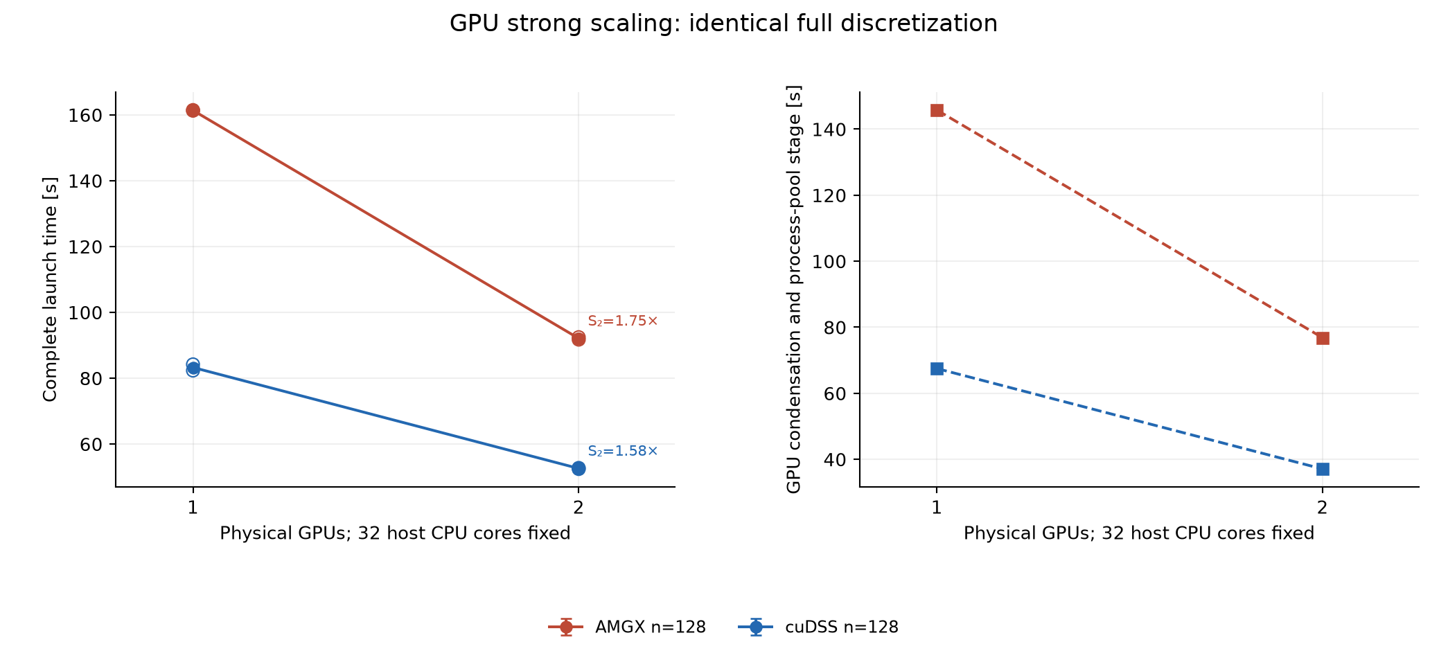
GPU strong scaling fixes the complete n=128 unit-cube discretization and 32 host CPU cores while varying one/two physical GPUs. The two panels distinguish the complete launch time from the GPU-process stage within the same acquisition.

Local solver	GPUs	Complete time [s]	GPU-process stage [s]	Self-speedup	Samples
cuDSS	1	83.26 [82.33, 84.18]	67.50	1.00	2
cuDSS	2	52.57 [52.42, 52.73]	37.07	1.58	2
AMGX	1	161.35 [161.26, 161.45]	145.78	1.00	2
AMGX	2	92.08 [91.72, 92.44]	76.82	1.75	2

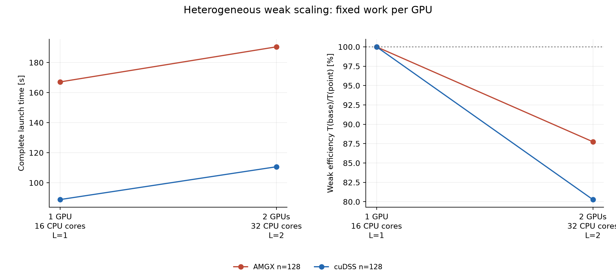
Heterogeneous weak scaling grows from one GPU with 16 host cores on L=1 to two GPUs with 32 host cores on L=2. Each GPU retains 64 macroelements and 16 host cores; local volume/trace resolution and material spatial period stay fixed. The one-GPU weak base has its own acquisition and CPU budget; it is not a relabeled 32-host-core strong sample. Its efficiency is Tbase/Tnext, without a factor two.

Local solver	1 GPU + 16 CPU, L=1 [s]	2 GPUs + 32 CPU, L=2 [s]	Weak efficiency [%]
cuDSS	88.83	110.65	80.3
AMGX	167.09	190.42	87.7

Complete cost, field accuracy and workflow phases

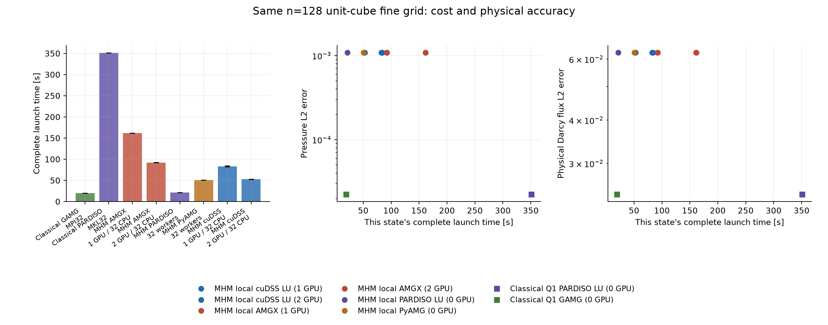
Matched-grid panels place complete workflow times beside pressure and physical Darcy flux errors. Every error marker uses that state's actual time and its own integrated field; timing bars use the stated configuration statistic. GPU configurations add their explicitly recorded devices to the host CPU budget.

n	Fine hexahedra	Classical CG/GAMG [s]	MHM PyAMG [s]	MHM cuDSS, 2 GPUs [s]	MHM AMGX, 2 GPUs [s]
128	2,097,152	19.68	50.63	52.57 [52.42, 52.73]	92.08 [91.72, 92.44]
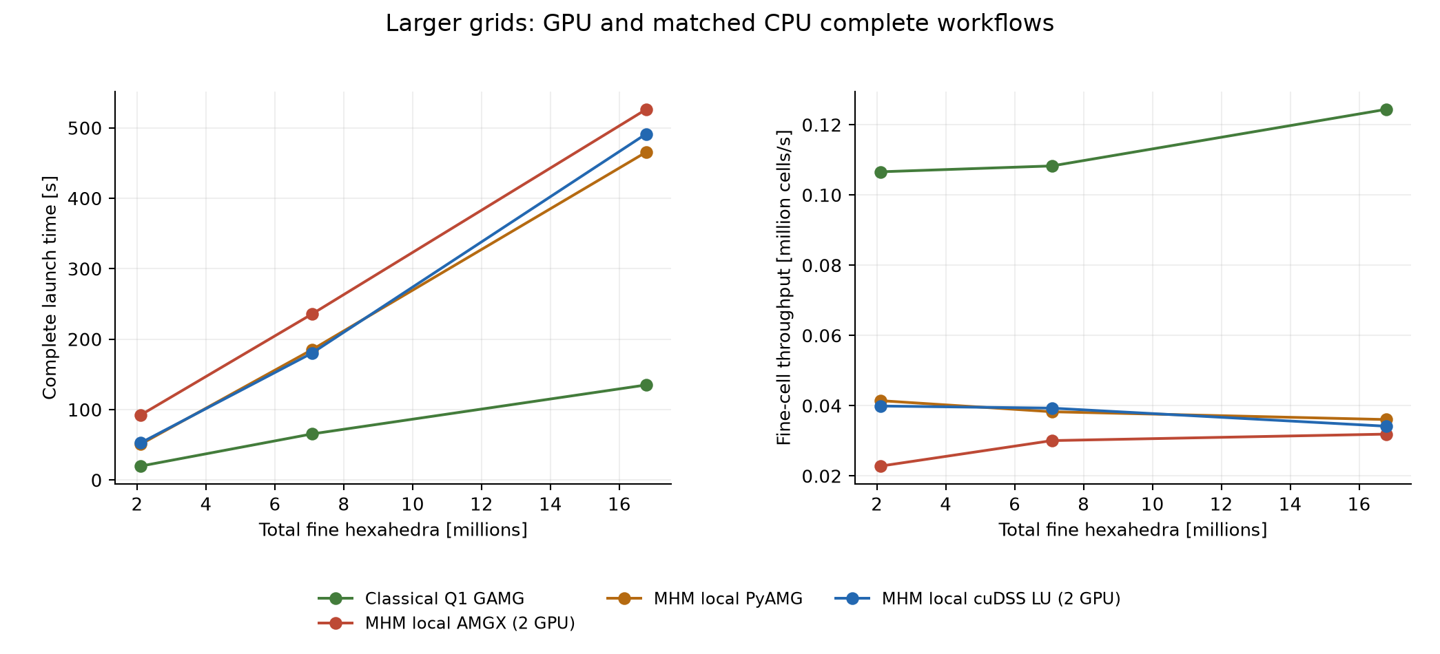
192	7,077,888	65.38	185.00	180.17	235.61
256	16,777,216	134.92	465.45	491.33	526.12

The classical distributed CG/GAMG workflow is faster than both GPU workflows on all three matched grids. At n=256, its complete time is 134.92s, compared with 465.45s for MHM PyAMG, 491.33s for MHM cuDSS and 526.12s for MHM AMGX. The two-GPU improvement relative to one GPU therefore does not establish a gain over the same-grid classical baseline.

n	Method	Actual raw SHA prefix	Actual raw time [s]	\(\lVert p_h-p_*\rVert_{L^2}\)	\(\lVert q_h-q_*\rVert_{L^2}\)
128	Classical Q1 GAMG	3e44ce886f	19.68	2.23180e-05	2.44114e-02
128	MHM local PyAMG	e96a7f6df5	50.63	1.08384e-03	6.26485e-02
128	MHM local cuDSS LU (2 GPUs)	0d6114a851	52.42	1.08384e-03	6.26485e-02
128	MHM local AMGX (2 GPUs)	10b3c1937a	91.72	1.08384e-03	6.26485e-02
192	Classical Q1 GAMG	18731d3e3b	65.38	9.92801e-06	1.63098e-02
192	MHM local PyAMG	2fdaacb2ec	185.00	1.08666e-03	5.99788e-02
192	MHM local cuDSS LU (2 GPUs)	d2e52126dd	180.17	1.08666e-03	5.99788e-02
192	MHM local AMGX (2 GPUs)	ae9771a328	235.61	1.08666e-03	5.99788e-02
256	Classical Q1 GAMG	7a585c500e	134.92	5.58630e-06	1.22418e-02
256	MHM local PyAMG	07dc7c38a3	465.45	1.08768e-03	5.90100e-02
256	MHM local cuDSS LU (2 GPUs)	8e21607648	491.33	1.08768e-03	5.90100e-02
256	MHM local AMGX (2 GPUs)	d1d1646c60	526.12	1.08768e-03	5.90100e-02

Each norm row above uses the first listed actual acquisition of that configuration, identified by its SHA prefix; its own clock is displayed separately from the configuration mean. The immutable JSON retains every repetition's own field norms and quadrature control. The fixed MHM macro/trace spaces retain the pressure-error floor while the classical fine-grid pressure error decreases.

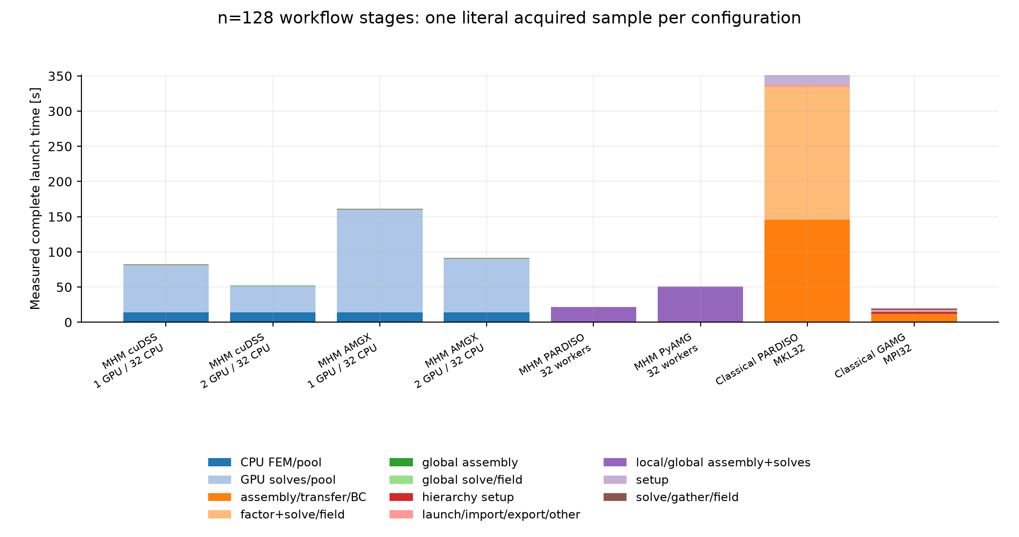
The phase plot stacks sequential parent-stage wall clocks from one literal acquired sample per configuration. It does not stack sums of parallel worker times. The clock remainder is labeled launch/import/export/other, rather than assigned to an unmeasured operation.

Larger local-grid experiments and scope

The larger-grid sweep fixes the unit cube, macro/trace spaces and two-GPU/host resource allocation while refining the local volume grid. It reports accepted absolute time and fine-cell throughput. This is a grid-size sweep, not weak scaling or an equal-accuracy comparison. A missing completed same-grid CPU reference has no assigned accelerator speedup.

These finite node-local observations do not establish asymptotic or multi-node scaling. The local/trace space distinction and fixed-trace pressure floor remain scientific limitations. Gomes et al. (2017, preprint v1) motivate independent MHM local work and CPU direct solvers; the present hexahedral manufactured application differs from their cluster experiment. Penna et al. (2019) motivate workload-aware scheduling; their reported gains are not assigned to this implementation.

Intel PARDISO, NVIDIA cuDSS and NVIDIA AMGX describe the native solver capabilities. Independent local device owners in this study differ from a distributed global-matrix GPU solver. Executed bindings, profiles and resources determine the verified scope of each recorded acquisition.

References

• Antônio Tadeu A. Gomes, Weslley S. Pereira, Frédéric Valentin, and Diego Paredes (2017). On the Implementation of a Scalable Simulator for Multiscale Hybrid-Mixed Methods, arXiv preprint, version 1, 30 March 2017. arXiv: 1703.10435v1.

• Pedro Henrique Penna, Antônio Tadeu A. Gomes, Márcio Castro, Patricia D.M. Plentz, Henrique C. Freitas, François Broquedis, and Jean‐François Méhaut (2019). A comprehensive performance evaluation of the BinLPT workload‐aware loop scheduler. Concurrency and Computation: Practice and Experience 31(18) e5170. DOI: 10.1002/cpe.5170.