Performance and parallel execution

The implementation separates local finite element assembly, local condensation, global sparse assembly and solution, and field reconstruction. A direct local solver reuses its constrained factorization for the source and skeleton lifts. The prepared GPU AMG solver reuses one hierarchy across its right-hand sides and original-equation corrections. A different material matrix requires a new setup. A HybridSystem retains the executed lifts for reconstruction.

Performance campaigns time their declared numerical workflow; bounded assembly controls state any untimed preparation. Numerical agreement and performance are verified separately: a faster execution must still satisfy the original equations and reproduce the physical fields at the stated accuracy.

Compiled array kernels

Selected scalar quadrature contractions, ordered contribution reduction and planar point-coordinate operations use cached Numba kernels. Local/global equations, providers and NumPy array contracts retain the same Python interface. Basix supplies finite-element tabulation; native DOLFINx assembly and external LU/AMG solvers keep their own compiled implementations. The standalone Darcy notebook shows explicit local/global equations, assembly, solution, physical fields and separate first/warm calls in two and three dimensions.

The ordinary scalar integration path uses binary64 with compensated tensor contractions and quadrature sums. It does not enable fastmath. Exceptional exponent ranges retain a guarded native-precision integration path; an intermediate overflow must not destroy a finite final operator entry. Explicit extended-precision solver/refinement inputs retain their separate contracts. The compiled leaves release the GIL but create no inner parallel pool. Shared macroface loads are accumulated by the ordered coordinator, preserving their addition order and conservation convention.

Numba specializes on first use and can cache its compiled code. These costs belong in first-call measurements; a warmed calculation alone does not describe startup. See the Numba compilation options and cache behavior.

First focused 2D and 3D campaign

The smooth manufactured problem has

\[ \begin{aligned} K(x)&=\exp\left(0.25\prod_{i=1}^d\sin(2\pi x_i/0.137)\right),\\ p_\star(x)&=\prod_{i=1}^d\sin(\pi x_i),\\ f&=d\pi^2Kp_\star-\nabla K\cdot\nabla p_\star. \end{aligned} \]

Continuous local P2 pressure and constant P0 macroface normal-flux traces are identical in both implementations. The material period is not aligned with macro translations; every local material matrix and factor is rebuilt. The reference is the package's original array implementation at revision 55359af7, with the same locked dependencies and acquisition helper. It is an implementation-equivalence baseline, distinct from a classical-method comparison.

Each complete timer includes geometry, description, native thread-limit setup, local assembly and factorization, ordered global reduction, global solution and reconstruction, analytical pressure/physical-flux norms, original-equation and macro-conservation controls, and named pressure samples. An isolated serial process uses one BLAS thread on the Xeon Silver 4216 workstation. Three fresh workflows follow the first call; only compiled code is reused. Imports and interpreter launch/exit are measured separately. Empty per-process Numba caches make compilation visible; no GPU transfers occur in this CPU campaign.

Case	Macroelements	Total local elements	Original warm median	Compiled warm median	Measured ratio
2D	32	2,048	4.408 s	4.180 s	1.054×
3D	48	3,072	13.644 s	12.604 s	1.083×

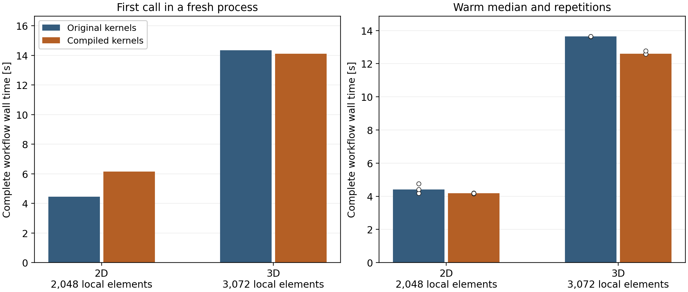
2D first workflow: 4.460 s original and 6.145 s compiled; 3D first workflow: 14.341 s original and 14.117 s compiled. First-call times include compilation and ordinary native initialization but exclude the separately recorded import/launch costs. The 2D repeated-time ranges overlap; the small median difference does not establish a general simulation speedup. The 3D result is also specific to this workload and machine.

Case	Pressure L2 error	Physical Darcy-flux L2 error	Original local L2 backward error	Macro skeleton balance
2D	0.036286	0.511646	2.77e-16	7.49e-15
3D	0.117950	0.939673	3.39e-16	5.55e-16

These P0 macroface controls are deliberately coarse. Their physical errors are reported as measured; they are not new high-accuracy or asymptotic convergence claims. Recorded pressure/trace differences between implementations remain at roundoff scale, with identical executed basis matrices and mesh coordinates. Original local equations and macro balance keep their unchanged 1e-10 limits. Macro conservation uses the skeleton normal flux, while the raw primal gradient flux is not claimed to conserve each fine cell. The notebook's field illustration uses explicitly enriched traces, separately from this fixed-space timing control.

Kernel gains and complete-workflow limits

The microbenchmarks exclude coefficient callbacks, tabulation, local solvers, physical norms and process startup. The diffusion inputs contain 384 synthetic cells, 36/64 quadrature points and six/ten basis functions in 2D/3D. The larger reduction consumes 1,024 SPD 25×25 blocks sharing 128 trace coordinates; actual MHM response blocks are timed separately.

Warm kernel ratio	2D inputs	3D inputs
Scalar diffusion Gram arrays	2.36×	1.77×
1,024 shared 25×25 blocks	5.51×	5.35×
Actual MHM contribution blocks	1.95×	2.23×

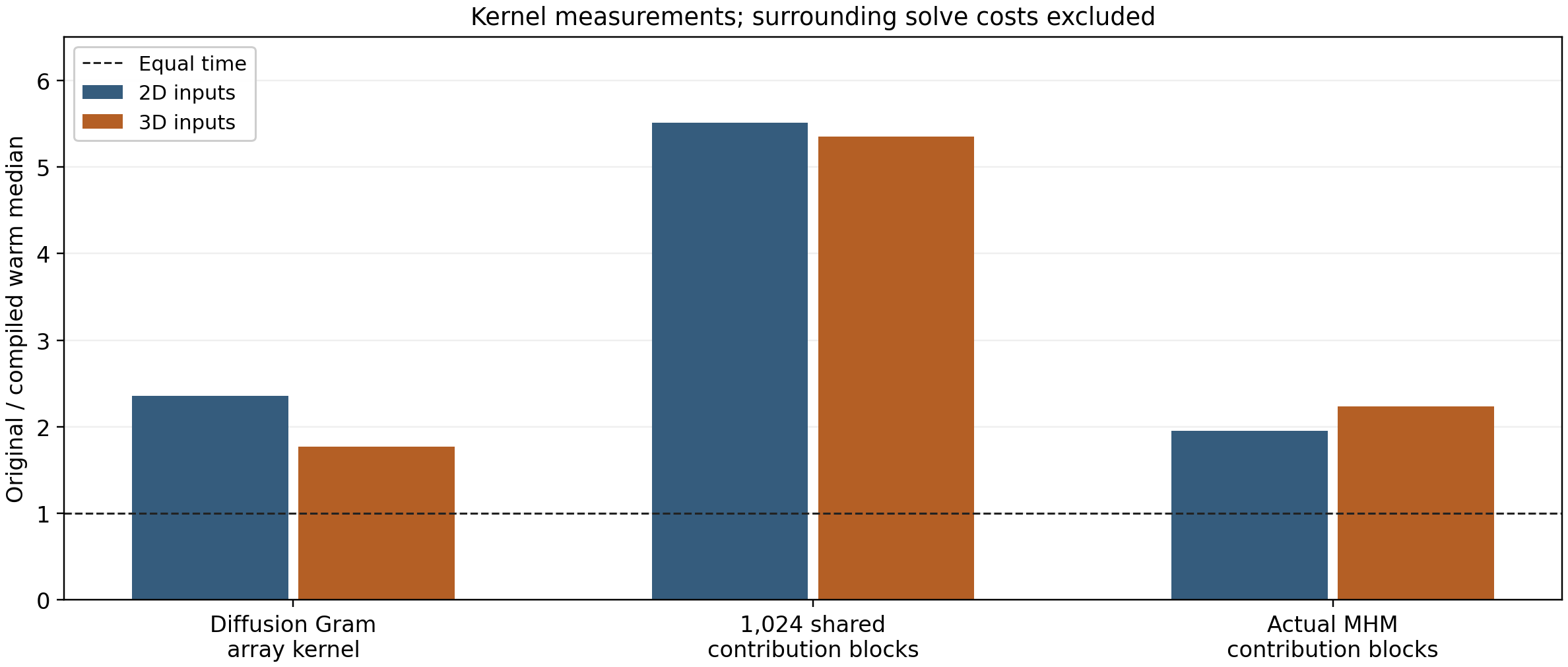
The shared-reduction matrix, RHS and absolute-load scale match exactly. Diffusion Gram differences are at binary64 roundoff scale. Planar point sampling has its own same-input geometric regression tests and timings; it is not a 3D locator optimization. These component gains do not predict an MPI/GPU speedup or a comparable gain for every PDE. Native tabulation, callback construction and other surrounding work remain significant in the complete simulations.

The complete report and raw repetitions include source/basis identities, package versions, CPU affinity, physical controls and separately measured launch costs. The importable acquisition helper owns timers and archives while delegating numerical operations to the package.

Cost of automatic native UFL trace assembly

The contextual API supplies numbering and orientation without user-managed maps. Its introductory native UFL pairings also change the boundary assembly route compared with explicit Basix trace matrices. A warmed serial control uses the same 4×4 macro mesh, Q2 fields, 4×4 fine cells per macroelement, piecewise P1 traces and oscillatory material in both routes. Three alternating repetitions measure:

Timed operation	Explicit Basix trace blocks	Contextual native UFL pairings
Description, local meshes, assembly, solution and one field sample	0.979 s	6.043 s
Native form lookup/binding, included above	0.561 s	5.186 s
Local condensation, included above	0.037 s	0.036 s
Global solution and recovery, included above	0.0027 s	0.0028 s

The observed timed-operation ranges are 0.975–0.994 s and 6.017–6.121 s. The native UFL route is 6.17× slower in this small workload, with 432 native form calls instead of 48. Independent trial/test pairings remain explicit. Repeated native form construction dominates; condensation and global solution retain their shared owners. Reusable native workspaces are available for explicitly prepared providers, while automatic reuse for these general contextual forms remains an optimization target.

Common macro geometry, data and callback definitions are prepared outside these timers. Both routes have an untimed warmup, one native thread and no concurrent project workload. Included timers overlap and are not additive. The route-cost receipt records every repetition, source snapshots, numerical equality checks, hardware and scope. This comparison changes the boundary assembly route as well as the API; it does not isolate Python abstraction overhead or predict large-problem scaling. The historical campaigns below retain their measured source revisions.

Oscillatory Darcy with declared local and global forms

The thread notebook defines its permeability, manufactured source, local UFL equations, skeletal couplings and conforming Q1 comparisons in executable cells. The process companion defines the same physical case and exports its displayed worker definitions for spawn. Their introductory workflow uses MeshHierarchy, bind_interface and bind_problem, with user-written LocalEquations and Equation forms. The scaling tables below retain their original measured source revisions and execution provenance. The notebooks verify archived records and execute a fresh field control by default; PYMHM_RUN_CAMPAIGN=1 requests new timing acquisitions.

Matched fine-element counts specify the amount of fine geometry; the global spaces differ. Separate pressure and physical-flux errors accompany timings. Native UFL checks precede timing. Timed volume assembly uses the verified Basix operators in both methods. Configurations are warmed before three randomized fresh solves, including setup, pool startup, transfers, ordered assembly, synchronization, the global solve and reconstruction. Operators, factors and AMG hierarchies are rebuilt for every solve.

On the two-socket Xeon Silver 4216 workstation, the thread campaign measured:

Fine quadrilaterals in each method	Classical LU	Classical AMG	Best MHM thread time	Workers
40,000	1.339 s	Not measured	2.358 s	1
250,000	8.484 s	Not measured	9.468 s	8
1,000,000	48.290 s	20.813 s	32.951 s	8

For one million elements, eight threads provide 2.125× speedup over one MHM thread and 1.466× over classical LU. Classical AMG is faster. Pressure and flux errors relative to the analytical solution agree within factors 1.003 and 1.001, respectively, between MHM and the conforming reference. The smaller workloads have no speedup against classical LU.

For one million fine quadrilaterals, the process companion measured:

Execution	Workers	Median complete time
MHM serial	1	69.531 s
MHM processes	1	81.504 s
MHM processes	4	24.772 s
MHM processes	8	17.140 s
MHM processes	16	13.287 s
Classical LU	1	48.181 s
Classical AMG	1	20.247 s

Sixteen processes provide 5.233× speedup over serial MHM, 3.626× over classical LU and 1.524× over classical AMG. Its three complete durations range from 13.243 to 13.428 s. Every configuration includes a fresh process pool where applicable; child imports, serialization and pool shutdown remain timed. Warm native initialization removes the common first-use cost from these medians, and the records also report that initialization separately. At 500×500 elements, eight processes take 6.153 s, compared with 8.118 s for classical LU and 4.540 s for classical AMG. Sixteen processes take 7.385 s; more workers do not improve that workload.

Weak scaling retains 40,000 local fine elements per worker on an expanding domain. Median complete time rises from 2.326 s with one thread to 292.479 s with 64 threads, giving 0.795% weak efficiency. These small local problems do not scale efficiently with threads. The process study measures its own startup and transfer costs on the physical domains [0, L] × [0, 1], with unchanged material period, source and boundary conditions:

Processes / domain length	Total fine elements	MHM processes	Classical LU	Classical AMG
1	40,000	3.691 s	1.043 s	0.745 s
4	160,000	5.778 s	4.616 s	2.954 s
8	320,000	9.704 s	10.318 s	6.277 s
16	640,000	14.631 s	20.074 s	12.025 s

Weak efficiency relative to one process is 25.229% at sixteen processes. Classical AMG remains faster on every weak workload. No inter-node efficiency follows from either one-host study.

The host has 32 physical and 64 logical cores. Native BLAS/OpenMP budgets are one thread, including the classical baselines. Project benchmarks run in separate timing windows; unrelated host applications remain active and there is no exclusive operating-system allocation or CPU affinity policy. Native initialization is recorded with the existing compiler cache, rather than as a cold-cache measurement. The thread records and figures and process records and figures contain every repetition, software versions, source and lockfile hashes, field checks and archived-basis replay conventions. This is an analytical application, rather than a matched reproduction of a literature experiment.

One- and two-GPU local condensation

The 500×500 pilot uses the same physical problem, 100 macroelements and 250,000 fine quadrilaterals with one or two NVIDIA RTX A5000 GPUs. Every MHM route compiles local equations on eight CPU threads, then condenses them with one CPU worker, eight CPU workers, one GPU or two GPUs. The CPU route with serial condensation therefore includes parallel compilation; it is not a complete serial MHM baseline.

All six routes run in the same locked hpc environment. Its SciPy version differs from the introduction environment used for the thread/process notebooks, so the pilot reruns classical LU and AMG in hpc. Each route has one warmup and three randomized fresh executions. Complete GPU timers include CPU setup and compilation, transfers, cuDSS analysis/factorization, synchronization, global assembly/solution and field reconstruction. Factors and responses are rebuilt for every execution.

Execution	Median complete time
MHM, serial CPU condensation	12.731 s
MHM, eight CPU condensation workers	9.932 s
MHM, one GPU	9.824 s
MHM, two GPUs	12.020 s
Classical LU	8.330 s
Classical AMG	4.521 s

The one-GPU and threaded CPU observed ranges overlap; their 1.1% median difference does not establish a performance advantage. Two GPUs are slower. Neither GPU route beats classical LU or AMG in this workload. Pressure and physical-flux errors agree with the classical baseline within factors 1.023 and 1.001. Original equations, physical moments and archived-basis replay are checked independently of timings.

The pilot records and figures include every sample, phase cost, initialization, actual basis digests and hardware/software provenance. CPU compilation and host analysis remain significant parts of this execution model. These measurements establish a node-local capability and its measured costs, without a multiGPU speedup or inter-node scalability claim.

Three-dimensional Darcy: workspaces, LU and AMG

The 3D tutorial shows the anisotropic material, exact fields, local/global UFL equations, oriented Q1 traces, independent references and native workspace provider. Compatible workers reuse mesh/space/kernel resources and buffers. Every macrocell assembles fresh material data and constructs independent LU factors or an AMG hierarchy; numerical responses are not cached. Material-independent trace/moment blocks are reused only after checking that property in the application forms.

The unit cube uses 64 macrohexahedra, with 262,144 or 884,736 total fine Q1 cells at counts 64 or 96 per unit direction. Four modes per unsplit macroface and one retained constant per cell give 1,024 coupled coordinates. Full pressure Dirichlet data impose no global mean-zero gauge. Pressure and broken physical flux are compared with exact fields; equal fine-element budgets do not imply equal global spaces or equal field accuracy.

Complete times include parent launch, imports/native initialization, setup, material assembly, fresh local solves, transfers, synchronization, global solution and reconstruction. Norm integration, archives and plots occur outside that timer. Warmups populate the existing compiler cache; cold JIT is not part of these measurements. Large parallel configurations have 32 physical cores and one native thread per process/rank.

Permeability spatial period, ε	Fine cells per unit axis	Method	Processes / ranks	Complete launch time (s)
0.1	64	Classical PETSc CG/GAMG	32	3.9623
0.1	64	Classical PETSc PREONLY/LU/MUMPS	32	16.8697
0.1	64	MHM MUMPS LU	32	5.1665
0.1	64	MHM PyAMG	32	8.2986
0.1	64	MHM SuperLU	32	6.0051
0.137	64	Classical PETSc CG/GAMG	32	3.7496
0.137	64	Classical PETSc PREONLY/LU/MUMPS	32	16.6027
0.137	64	MHM MUMPS LU	32	5.0159
0.137	64	MHM PyAMG	32	7.9710
0.1	96	Classical PETSc CG/GAMG	32	9.2592
0.1	96	Classical PETSc PREONLY/LU/MUMPS	32	96.3061
0.1	96	MHM MUMPS LU	32	10.4146
0.1	96	MHM PyAMG	32	22.5916
0.1	96	MHM SuperLU	32	56.0215

At matched 32-physical-core and fine-element budgets, local MUMPS MHM is 3.27× faster than classical distributed MUMPS at 64 cells per unit axis and 9.25× faster at 96. The period-0.137 LU comparison gives 3.31×. These are measured workflow ratios for different approximation spaces, with the physical errors shown alongside them. They are not equal-accuracy speedups.

Classical distributed CG/GAMG remains faster than both MHM local MUMPS and MHM local PyAMG at the measured unit-cube resolutions. The favorable LU comparison therefore does not establish an advantage over the best classical solver measured here. Each timing point is an actual completed sample; no confidence interval or variance estimate is inferred.

The six-point period-0.1 strong studies use 1, 2, 4, 8, 16 and 32 spawned processes. Focused weak studies keep four or eight macrocells per process, expanding the x-domain while preserving H=0.25, h=1/64 and the material wavelength. Their actual smallest measured process count supplies the weak efficiency baseline. Startup and the growing global skeleton limit these node-local measurements; no asymptotic or multi-node efficiency is inferred.

The case page displays complete-time, speedup, efficiency, phase-cost and focused weak plots, together with physical errors. The record and figures contain the actual measured samples and independent numerical controls. Periods 0.1 and 0.137 remain separate. Fixed Q1 macro traces leave an interface error floor when only local meshes are refined. Classical CG/GAMG remains faster in these measured cases. The separate CPU PARDISO and GPU edition extends the study with larger grids, one/two-GPU measurements and focused CPU/GPU weak scaling. Each edition retains its own measured configurations and numerical controls. Its numerical records and figures include each acquisition's own pressure and physical-flux errors.

Choosing and measuring an execution mode

Use assemble(problem, execution=ExecutionConfig(...)) with declared local and global forms. Serial execution builds, condenses and accumulates one cell at a time. Process execution constructs and reduces complete local equations inside spawned workers; ordered coordinator reduction handles shared faces. A bounded rolling window can overlap local work with global accumulation. The execution guide specifies ordering, thread limits, failure handling and cleanup.

Keep the full discretization fixed for strong scaling. For weak scaling, report both local work per worker and growth of the global skeleton. Retained lifts, serialized responses and the host global matrix all contribute to memory use. Separate initialization, local assembly/condensation, transfers, global work and reconstruction, while retaining a complete timer containing every phase. Report every repetition and any regression.

Ordinary MultiscaleProblem assembly has a host global solve. For distributed local ownership and global sparse algebra, use solve_distributed, with the caller assigning cells and globally consistent trace indices to MPI ranks. For node-local accelerator work, condense_multi_gpu distributes local systems among explicitly selected devices. Transfers, synchronization and host work remain part of a complete GPU comparison. Native correctness controls and one-host measurements do not establish multi-node efficiency.

Recorded MPI, resident GPU and offline/online measurements state their own hardware, spaces and timing scopes. Earlier CPU measurements remain available in the benchmark records. Their measured workloads and acquisition hashes are distinct from the oscillatory application above.

Additional 3D CPU and accelerator component measurements report their own CPU allocations, solver settings and timing scopes.