Adaptive macro refinement and work

Executable notebook · Download notebook

This lesson uses the estimator of Barrenechea et al. (2026) on a smooth localized exact pressure. The uniform studies in the recovery and indicator lessons first verify their asymptotic estimates. Here eight actual adaptive solves test the marking/refinement workflow and compare the same physical error against work.

1. Define a localized physical solution

\[ p(x,y)=x(1-x)y(1-y)\exp\!\left[-80\big((x-0.3)^2+(y-0.4)^2\big)\right]. \]

The pressure vanishes on every boundary edge. Set \(K=I\), \(q=-\nabla p\), and \(f=-\Delta p\). The notebook writes the NumPy derivatives explicitly and derives the UFL source from the analytical expression independently. This is an analytical extension of the paper's estimator examples, rather than a reproduction of its heterogeneous-material application.

def localized_forcing(domain):
    """Differentiate the analytical UFL pressure independently of NumPy."""
    x = ufl.SpatialCoordinate(domain)
    p = x[0]*(1-x[0])*x[1]*(1-x[1])*ufl.exp(-80*((x[0]-.3)**2+(x[1]-.4)**2))
    return -ufl.div(ufl.grad(p))

2. Declare the local and global variational equations

Reuse the explicitly written UFL volume and trace equations from the recovery lesson. Choose P3 local pressure, independent P1 normal traces, RT2 reconstruction, two local edge subdivisions and the physical constant volume moment. Only the source expression changes; the method and polynomial degrees remain fixed.

\[ \begin{aligned} (\nabla p_T,\nabla v)_T+\langle\lambda_T,v\rangle_{\partial T}&=(f,v)_T,\\ -\sum_T\langle p_T,\mu_T\rangle_{\partial T}&=0. \end{aligned} \]

3. Assemble, solve and measure before marking

Start with 32 macrotriangles. Rebuild the same declared forms after each refinement. solve_declared in the notebook merely orchestrates those already written forms and caller-chosen spaces; it does not select a Darcy formulation.

adaptive_mesh = TriangleMesh.unit_square(4)
for step in range(8):
    solution = solve_declared(adaptive_mesh, 1, localized_source, localized_forcing)
    estimate = estimate_darcy_error(
        solution, homogeneous_dirichlet=True, degree=2, quadrature_order=16,
    )
    energy_error = estimate.energy_error(localized_gradient, order=16)
    assert estimate.total >= energy_error
    marked = mark_dorfler(estimate.local_squared, theta=0.5)
    if step < 7:
        adaptive_mesh = refine_triangles(adaptive_mesh, marked).mesh

For budget-based refinement, refine_darcy_budget preserves the Dörfler bulk set and conforming closure; the resulting macro-cell count may exceed the requested budget.

The acquisition additionally integrates each physical error at orders 12 and 16 and checks original global compatibility and continuous-test equilibrium at every cycle. A separate native eight-subdivision control verifies all original local volume/trace rows for this localized pressure: maximum local relative defect \(4.20\times10^{-15}\) and full uncondensed defect relative to the physical load \(6.12\times10^{-15}\). These algebraic checks use the unchanged \(10^{-10}\) gate; they do not replace the physical-error study. The mesh owner performs conforming closure; refining only the selected triangles without this closure would not satisfy the estimator's mesh hypotheses.

4. Distinguish marking from the chosen discretization control

Dörfler marking satisfies

\[ \sum_{T\in\mathcal M}\eta_T^2\ge\theta\sum_T\eta_T^2,\qquad\theta=\tfrac12. \]

This study refines the macro partition and rebuilds local meshes. Local mesh refinement changes the local approximation; trace segmentation changes the skeleton space. Each choice requires compatible degrees and partitions. Refinement ancestry is available for preserving material and boundary markers.

5. Compare adaptive error against a matching uniform sequence

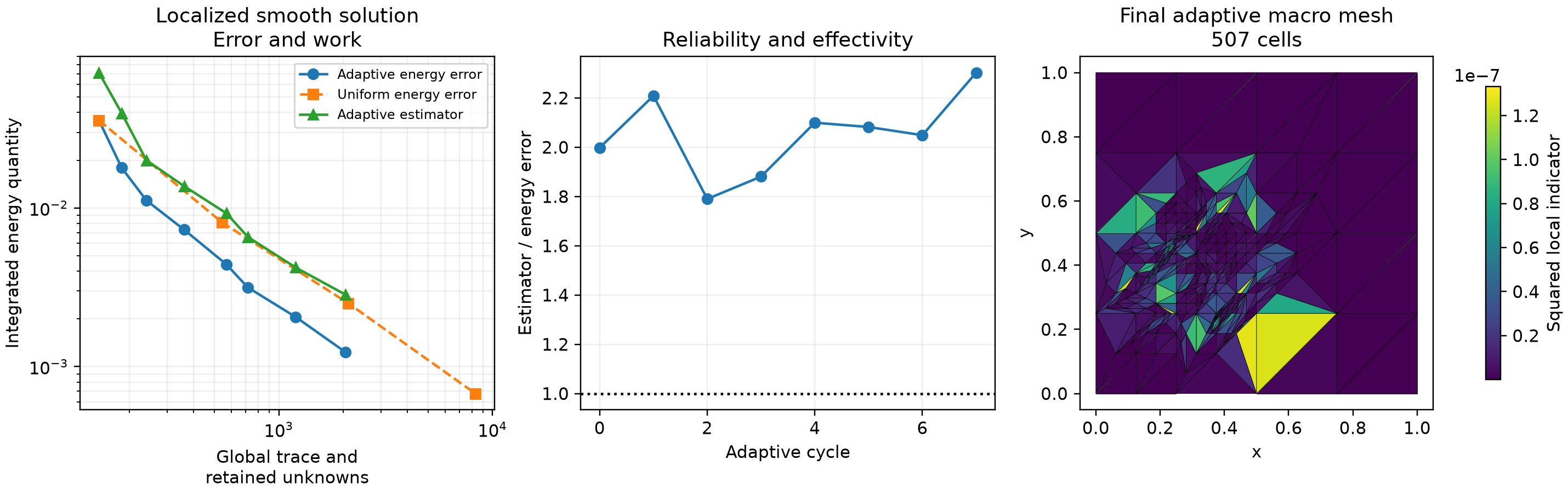
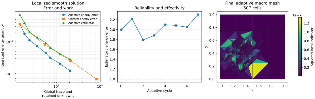
Uniform P3/P1/RT2 calculations use the same localized pressure, coefficient, source, boundary conditions and local mesh ratio on \(n=4,8,16,32\). Work counts trace plus retained mean unknowns. The adaptive horizontal coordinate is not a single fictitious mesh size; no uniform-grid exponent is fitted to it.

PDF · SVG

Adaptive cycle	Macrotriangles	Global trace + mean unknowns	Energy error	Effectivity
0	32	144	3.570890e-02	1.9984
1	42	184	1.792702e-02	2.2090
2	56	240	1.117302e-02	1.7902
3	86	360	7.311391e-03	1.8809
4	138	568	4.415988e-03	2.0999
5	175	717	3.152546e-03	2.0823
6	295	1197	2.060652e-03	2.0491
7	507	2045	1.237290e-03	2.3031

The last adaptive mesh has 2,045 global unknowns and energy error \(1.23729\times10^{-3}\). The matching uniform 16-subdivision mesh has 2,112 unknowns and error \(2.51067\times10^{-3}\): a factor of 2.03 in physical error at comparable global work. A smaller physical error at comparable work is the relevant measured adaptive benefit. The estimator is checked against the exact energy error at every cycle. Its nonconformity and divergence terms are retained throughout.

PDF · SVG

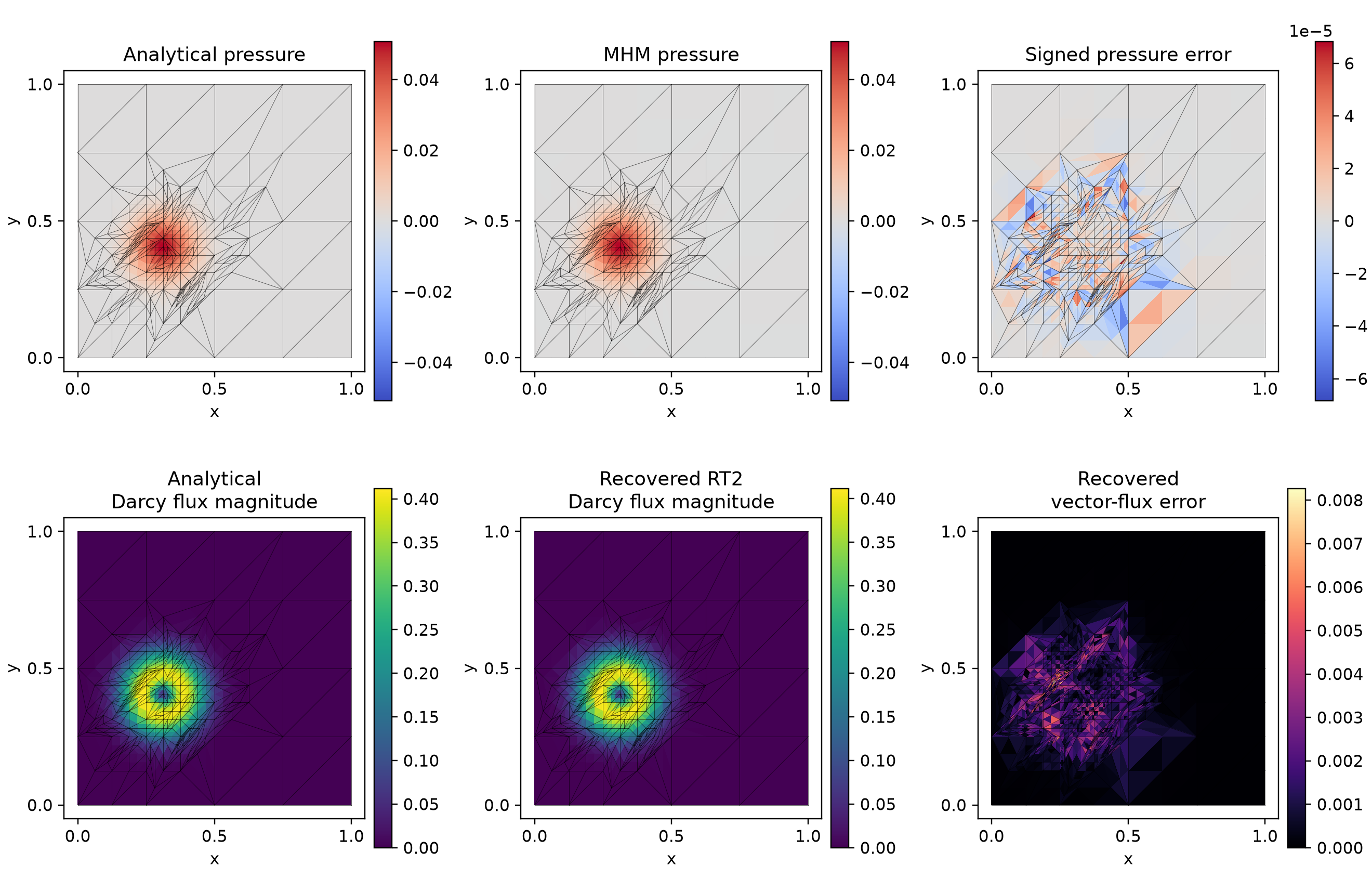
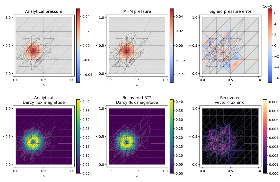
Field/error panels preserve the actual macro partition and independent one-sided values. These centroid display samples are separate from physical volume integration. The independently assembled classical reference below uses exactly this localized source, coefficient and boundary data. The analytical pressure remains the exact comparator for all reported physical norms.

6. Verify a matching classical Galerkin reference

The global reference assembles a continuous P3 Galerkin space independently of MHM. Its weak formulation has exactly the same identity coefficient and localized source. The UFL source is derived from the analytical pressure above:

def reference_forms(domain, V):
    p, v = ufl.TrialFunction(V), ufl.TestFunction(V)
    dx = ufl.Measure("dx", domain=domain, metadata={"quadrature_degree": 20})
    return (ufl.inner(ufl.grad(p), ufl.grad(v))*dx,
            localized_forcing(domain)*v*dx)

Use the notebook's explicitly defined localized_pressure and localized_gradient callbacks for the analytical comparison. The boundary selector below imposes the same zero pressure on all four sides. Execute all three reference meshes with the same forms and degree:

from examples.tutorial_recovery_reference import classical_reference_control


def boundary_nodes(points):
    """Select the homogeneous boundary values on the unit square."""
    return np.flatnonzero(np.any(np.isclose(points, 0) | np.isclose(points, 1), axis=1))


classical_rows = []
for n in (32, 64, 128):
    with threadpool_limits(1):
        row, reference_field = classical_reference_control(
            TriangleMesh.unit_square(n), 3, reference_forms, boundary_nodes,
            localized_pressure, localized_gradient,
        )
    row["mesh_resolution"] = n
    classical_rows.append(row)
    print(n, row["scalar_l2"], row["flux_l2"], row["quadrature_relative_difference"])

Native mesh/space mapping, essential elimination and independently integrated physical norms use the reusable acquisition owners in the reference helper. The caller supplies the mesh, degree, these variational forms, boundary-node indices and analytical pressure/gradient. No local MHM matrix or coefficients are passed to the global reference.

The three refined reference meshes give:

Global square subdivisions	P3 nodal unknowns	Pressure error	Physical vector-flux error
32 × 32	9409	3.490465e-07	1.126836e-04
64 × 64	37249	2.150600e-08	1.414326e-05
128 × 128	148225	1.338314e-09	1.769402e-06

Pressure orders are 4.021 and 4.006; physical-flux orders are 2.994 and 2.999. Both norm rules agree to a maximum relative difference of 5.45e-12.

PDF · SVG

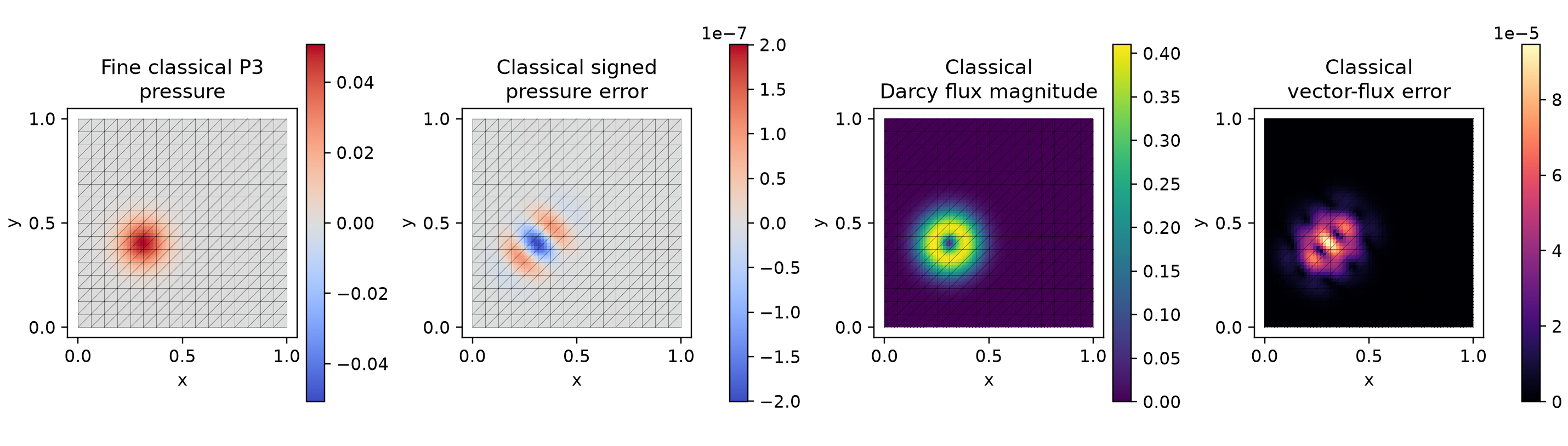
The reference fields use the 64-subdivision global mesh. The overlay is the 16-subdivision uniform comparison macro mesh, rather than the adaptive mesh. Every pressure/flux error shown compares the same analytical localized fields.

Reproduce this tutorial

The notebook linked at the top defines the forms and runs the recovery, indicator, adaptive and recursive studies. Install the native notebook backend as described in the installation guide, then open it from the source checkout:

pixi run --locked -e introduction jupyter lab notebooks/darcy/reconstruction_and_indicators.ipynb

References

• Gabriel R. Barrenechea, Larissa Martins, Weslley Pereira and Frédéric Valentin (2026). An H(div; Ω)-Conforming Flux Reconstruction for the Multiscale Hybrid-Mixed Method, Multiscale Modeling & Simulation 24(2), 399–428. DOI: 10.1137/24M1673073; accepted author manuscript.
• Christopher Harder, Diego Paredes and Frédéric Valentin (2013). A family of Multiscale Hybrid-Mixed finite element methods for the Darcy equation with rough coefficients, Journal of Computational Physics 245, 107–130. DOI: 10.1016/j.jcp.2013.03.019.