Comparisons with published results

The four Darcy error curves in Figure 5 of Harder, Paredes and Valentin (2013) are matched at five resolutions by classical RT0/P0 fluxes and their integrated quadratic potentials: the largest discrepancy from the digitized figure is 0.20%. The primal P1 discretization gives different values. The comparisons below distinguish these local approximations on the same meshes. The separate analytical MHM campaign retains the source correction in equation (42) and reconstructs the nonconstant-source Neumann lifting. Its coarse pressures differ from classical RT0. Agreement with the classical curve does not establish reproduction of the full-source MHM formulation.

Stokes P2/P2 locals with constant traces match four Figure 3 curves at six levels within 0.14%. P3/P3 with linear traces matches three Figure 4 curves at six levels within 0.70%. The full pseudostress L2 diagnostic remains inconsistent with the plotted ordinate; both the evidence and the distinct H(div) norm conventions are reported below. Published Brinkman conservation data and a flux-reconstruction table are reported with their comparison scope.

The numerical fields on this page are computed by pyMHM: native RT0/P1 operators for Darcy and DOLFINx/UFL local assembly for the higher-order Stokes examples. The comparison values come from the articles' tables or digitized figures. These runs do not execute the historical programs that produced those figures. The separate MSL code comparison and NeoPZ code comparison compare independently executed implementations.

Published datasets and digitization

Numerical tables retain their printed precision. For the three digitized figures, vector path coordinates are calibrated against logarithmic axis ticks; visible markers and legends identify the series. Rendered pages provide the visual reference for table and figure transcription. The chosen comparison tolerance is 1% for these digitized ordinates. It is an analyst's allowance for figure extraction, not a statistical confidence interval or a statement about the authors' solver accuracy.

The repository's examples/results/published/ directory contains:

Dataset	Source and location	Nature of the numbers
harder2013_figure5.csv	JCP 245, Figure 5, printed p. 117; PDF p. 11	Four curves, five digitized points each
araya2017_figure3.csv	CMAME 324, Figure 3, printed p. 42; PDF p. 14	Five Stokes error curves, six digitized points each
araya2017_figure4.csv	CMAME 324, Figure 4, printed p. 42; PDF p. 14	Five Stokes error curves for linear traces, six digitized points each
araya2017_table1.csv	CMAME 324, Table 1, printed p. 43; PDF p. 15	Stokes macrocell mass defects
araya2017_table2.csv	CMAME 324, Table 2, printed p. 44; PDF p. 16	Brinkman macrocell mass defects
barrenechea_reconstruction_manuscript_table2.csv	Author manuscript, Table 2, printed/PDF p. 23	Energy error and estimator components

provenance.json records titles, authors, DOI identifiers, source-version checksums, extraction methods, norm definitions and unresolved parameters. Decimal places in digitized CSV files preserve the extraction output; they must not be interpreted as equally many significant experimental digits.

Darcy 2013: Figure 5

Problem and spaces

Section 5.1 prescribes, on \(\Omega=(0,1)^2\),

\[ K=I,\qquad p=\cos(2\pi x)\cos(2\pi y),\qquad f=8\pi^2p,\qquad q=-\nabla p. \]

The entire boundary has homogeneous outward Neumann flux, and the pressure has zero mean. These conditions differ from the cosine-\(\pi\) Dirichlet problem in the other Darcy gallery.

Figure 5 uses degree-zero face traces. The text specifies structured triangular meshes. Page 119 states that second-level computations use one element with polynomial degree \(\ell+1\), which gives P1 for \(\ell=0\). However, equation (40), page 114, gives exact quadratic radial lifts for this same constant coefficient, degree-zero case; their gradients are RT0 fields. Section 4.1.1 and the discussion immediately preceding Figure 5 invoke this RT0 equivalence. Consequently, the paper supplies two different local-space descriptions relevant to this experiment. The numerical evidence below discriminates between them, but cannot identify the original code path by itself.

Our declared mesh consists of \(n\times n\) equal squares, each split from its lower-left corner to its upper-right corner. It contains \(2n^2\) triangles. The grid spacing is \(s=1/n\), while the maximum geometric triangle diameter is \(H=\sqrt{2}/n\). The paper formally defines its mesh parameter as a maximum diameter, yet the graph's five abscissas are approximately \(1/4,1/8,1/16,1/32,1/64\); its exact connectivity and relation to a grid count are not supplied. We therefore pair these labels with the declared grid spacing for the comparison and retain both spacing and diameter in the result files. The P1 and RT0 comparisons use the same mesh.

Both runs use one fine triangle per macrocell, constant face traces, source integration with Duffy order 10, and error integration with order 12. Increasing these to orders 12 and 14 on the coarsest grid changes the measured norms by less than \(2\times10^{-13}\) relatively. The article does not specify its quadrature rules.

Four separate norms

Let \(p_0\) be the coarse constant in each macrocell and let \(\Pi_0p\) be the cell-average projection of the analytical pressure. The four curves are

\[ \|p-p_h\|_{L^2},\quad \|q-q_h\|_{L^2},\quad \|p-p_0\|_{L^2},\quad \|\Pi_0p-p_0\|_{L^2}. \]

The coarse coefficients are taken directly from the hybrid solution and checked against reconstructed cell means. All norms are absolute, not divided by the corresponding exact-solution norm. Equation (34) and the Figure 5 legend use \(\sigma(p_h)=-K\nabla p_h\); no separate flux-averaging step is specified for this figure. The vertex averaging mentioned in Section 5.2 concerns a different five-spot visualization.

Published nominal h	Updated pressure L2	Flux L2	Coarse pressure L2	Projected coarse pressure L2
1/4	0.122294	2.03857	0.249585	0.0576425
1/8	0.0316637	1.01279	0.129654	0.0178403
1/16	0.00799107	0.504787	0.0653440	0.00470828
1/32	0.00199988	0.252003	0.0327241	0.00119070
1/64	0.000500474	0.125997	0.0163621	0.000299251

Primal P1 approximation

Primal P1 pressure gives the measured refinement orders below, but its gradient is constant on each triangle. Its values differ systematically from the published curves, beyond the digitization tolerance.

At \(n=64\), relative differences from the digitized ordinates are −2.87% for updated pressure, +28.98% for flux, −0.025% for coarse pressure and −55.36% for projected coarse pressure. The last observed refinement orders are respectively 1.998, 0.999, 0.999 and 1.991. Correct orders alone therefore do not demonstrate numerical reproduction. The full P1 record preserves all five levels and the discrepancies.

Classical RT0 and quadratic pressure

For unit permeability, an RT0 flux on one triangle has the form

\[ q_h(x)=q_h(c_T)+b_T(x-c_T),\qquad b_T=\frac12\nabla\cdot q_h, \]

where \(c_T\) is its centroid. Integrating this field and imposing the same coarse mean \(p_{0,T}\) gives the unique quadratic radial potential

\[ p_T^\star(x)=p_{0,T}-q_h(c_T)\cdot(x-c_T) -\frac{b_T}{2}\left(|x-c_T|^2- \frac1{|T|}\int_T|z-c_T|^2\,dz\right). \]

It satisfies \(-\nabla p_T^\star=q_h\) and \(\Pi_0p_T^\star=p_{0,T}\). The second moment used here is \(\frac1{12}\sum_{i=1}^3|v_i-c_T|^2\), for triangle vertices \(v_i\). This construction uses the computed RT0 flux and mean pressure; it contains no fitted constants or adjustment to the published errors. Its polynomial form is the one identified by the exact lift in equation (40).

The native mixed pressure remains P0. The updated-pressure curve below uses \(p_T^\star\), explicitly distinguished from that native P0 variable.

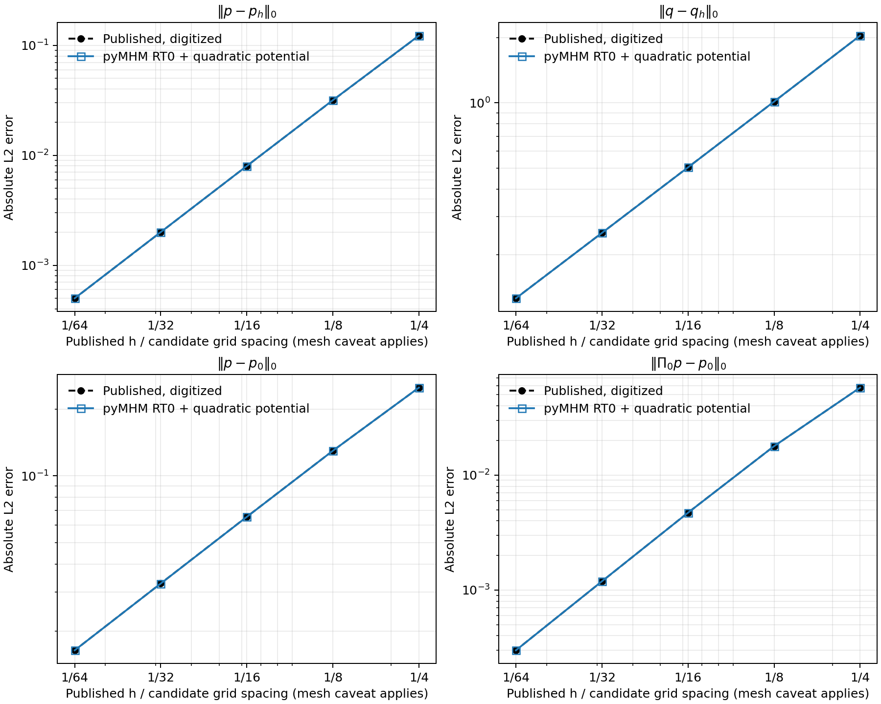
n	Quadratic pressure L2	Flux L2	Coarse pressure L2	Projected coarse pressure L2
4	0.122537	2.03845	0.249615	0.0576301
8	0.0317066	1.01311	0.129650	0.0178377
16	0.00799234	0.504483	0.0653054	0.00470480
32	0.00200216	0.251935	0.0327073	0.00119201
64	0.000500793	0.125927	0.0163603	0.000298999

Across all five levels, maximum absolute relative discrepancies are 0.199%, 0.0602%, 0.0591% and 0.1102%, respectively. All twenty comparisons pass the declared 1% digitization tolerance. The mixed comparison record also retains the native P0 pressure error, separate from the quadratic one.

The source lifting also distinguishes the discrete formulations. This single-cell RT0 field has \(\nabla\cdot q_h=\Pi_0f\), and its quadratic potential satisfies \(-\Delta p_T^\star=\Pi_0f\). The exact source lifting in equation (29) instead solves for \(f-\Pi_0f\) with zero normal flux. It vanishes for a cellwise constant source, but the cosine source is not cellwise constant. Moreover, equation (42) contains a source-dependent load correction relative to the classical RT0 method. The native RT0/P0 solve does not insert that extra correction. The observed match concerns the plotted numerical values within figure resolution. The full-source analytical MHM provides the separate six-level comparison using the source term as written in equation (42). The original treatment of that term and the precise mesh-parameter convention remain unconfirmed.

Darcy numerical records

The five-level records are preserved in examples/results/darcy_2013_comparison.json and examples/results/darcy_2013_mixed_comparison.json. The notebook 11_published_darcy_2013.ipynb presents the archived levels and figures alongside their discretization and interpretation. The public plotting command at the end of the Stokes comparison renders both Darcy and Stokes records.

Stokes 2017: equal-order local spaces and direct figure comparison

Araya et al. (2017), Section 3.1.1, uses one triangle per local problem and USFEM equal-order spaces \(P_{\ell+2}^2/P_{\ell+2}\). The comparison assembled these spaces through DOLFINx/UFL using from_ufl, and solved the skeleton problem through pyMHM's HybridSystem. The preserved results cover P2/P2 with constant traces at six levels and P3/P3 with linear traces at six levels. Refined P1/P1 USFEM and Taylor–Hood P2/P1 are different approximations and are not substituted for these published spaces.

The Stokes data are \(\nu=1\), \(\gamma=0\),

\[ \begin{aligned} u_1&=-256x^2(x-1)^2y(y-1)(2y-1),\\ u_2(x,y)&=-u_1(y,x),\\ p&=150(x-1/2)(y-1/2). \end{aligned} \]

The velocity vanishes on the square boundary; pressure has zero mean. The forcing is \(-\Delta u+\nabla p\). Using the streamfunction \(\psi=-128x^2(x-1)^2y^2(y-1)^2\) and \(u=(\partial_y\psi,-\partial_x\psi)\) preserves exact incompressibility.

Discretization, geometry and stabilization

Each of the \(n^2\) squares is split into four triangles by its center. The resulting crisscross mesh has \(4n^2\) triangles, maximum diameter \(H=1/n\) and shorter triangle sides \(H/\sqrt2\). The same mesh family is generated by MSL's msl_core and exercised by its msl_mhm Darcy driver in the MSL code comparison. This supports the mesh choice but does not identify the exact connectivity used for the Stokes article. The paper does not supply its connectivity explicitly. Figure 3's abscissas are approximately \(H/\sqrt2\), whereas Table 1 and Figure 4 use \(H\). Both coordinates are retained in the digitized datasets; the comparisons below pair the ordered levels with Table 1. No horizontal translation is optimized against the errors.

A separate comparison uses two triangles per square. It produces different errors, including pressure L2 error 4.60146 at \(n=4\), versus 3.15562 on the crisscross mesh. Replacing one connectivity by the other changes the experiment; matching local degree alone is insufficient.

For the Stokes limit of equations (41)–(42), the local stabilization coefficient is

\[ \tau_T=\frac{m_T h_T^2}{8\nu},\qquad m_T=\min(1/3,C_T),\qquad C_T h_T^2\|\Delta v_h\|_T^2\leq\|\nabla v_h\|_T^2. \]

The example calculates the largest admissible \(C_T\) from the generalized eigenproblem for the polynomial Laplacian and gradient matrices, after quotienting constants. This gives \(C_T=1/96\) for P2 and \(C_T=0.003353888994497343\) for P3 on the right isosceles triangles. For P2 the value also follows analytically: the two eigenvalues of the triangle's coordinate covariance are \(h_T^2/24\) and \(h_T^2/72\), so the sharp Laplacian-to-gradient ratio is \(96/h_T^2\). These constants are derived from the inequality; they are not fitted to published errors. The paper's numerical subsection does not state the constant used by its implementation.

The UFL forms implement

\[ \begin{aligned} a_T((u,p),(v,q))={}&(\nabla u,\nabla v)_T-(p,\nabla\!\cdot v)_T -(q,\nabla\!\cdot u)_T\\ &-\tau_T(-\Delta u+\nabla p,-\Delta v+\nabla q)_T,\\ L_T(v,q)={}&(f,v)_T-\tau_T(f,-\Delta v+\nabla q)_T. \end{aligned} \]

The pressure-test sign is the symmetric convention obtained by changing \(q\) to \(-q\) in the article's mixed form. The local nullspace contains the two velocity translations; zero local velocity means fix those modes. A single global mean-pressure constraint fixes the pressure gauge. Degree-16 quadrature integrates the polynomial data and squared errors; a separate degree-18 check at \(n=4\) agrees to floating-point precision.

P2/P2, constant trace: six levels

n	Triangles	Velocity L2	Velocity H1 seminorm	Pressure L2	Standard broken stress H(div)
4	64	0.227692	3.53312	3.15562	12.6128
8	256	0.0665358	1.87579	1.37434	6.18796
16	1024	0.0175635	0.960272	0.615813	3.06202
32	4096	0.00446662	0.483943	0.291503	1.52462
64	16384	0.00112246	0.242571	0.142683	0.761191
128	65536	0.000281046	0.121376	0.0708286	0.380414

All 24 ordinates across these four curves agree with digitized Figure 3 within the declared 1% extraction tolerance. Maximum discrepancies are 0.1392% for velocity L2, 0.1324% for its H1 seminorm, 0.1107% for pressure L2, and 0.0519% for the standard broken H(div) norm. All six published levels are included. Its stress L2 curve and the written H(div) weighting require the separate qualification immediately below.

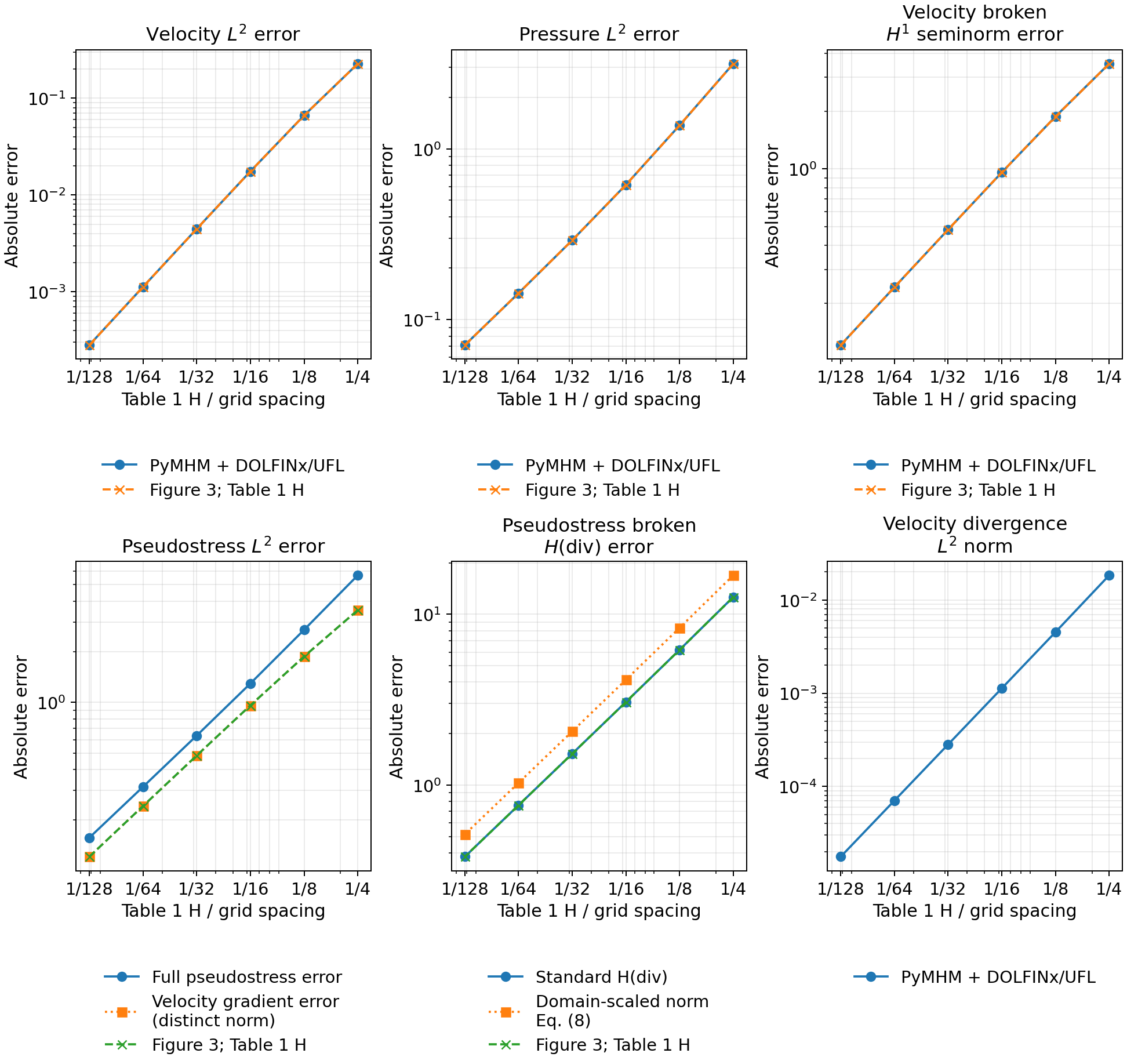
The pressure is plotted independently on each macrotriangle, preserving jumps. Outlined edges identify the actual macro partition on every field panel. The smooth-looking analytical pressure is not used to interpolate the numerical solution. The last panel shows sampled pointwise errors; it is not the integrated L2 error in the table. Download the scalar results and all published-value comparisons.

P3/P3, linear trace: six levels

n	Velocity L2	Velocity H1 seminorm	Pressure L2	Standard broken stress H(div)
4	0.00822259	0.284419	0.198787	5.14833
8	0.000982929	0.0711466	0.0471099	2.5453
16	0.000123603	0.0180124	0.0110797	1.235
32	1.57303e-05	0.00456664	0.00266962	0.604656
64	1.9916e-06	0.00115218	0.000653952	0.298658
128	2.50777e-07	0.000289530	0.000161735	0.148347

The three velocity/pressure curves of Figure 4 agree at all eighteen compared points: the maximum discrepancy is 0.6935%, below the same 1% digitization allowance. The observed reductions are approximately third order for velocity L2 and second order for pressure L2 and velocity H1. All six published levels are included. The stress H(div) curve differs by up to 10.03%; that difference is retained, together with the unknown historical inverse constant and stress diagnostic convention.

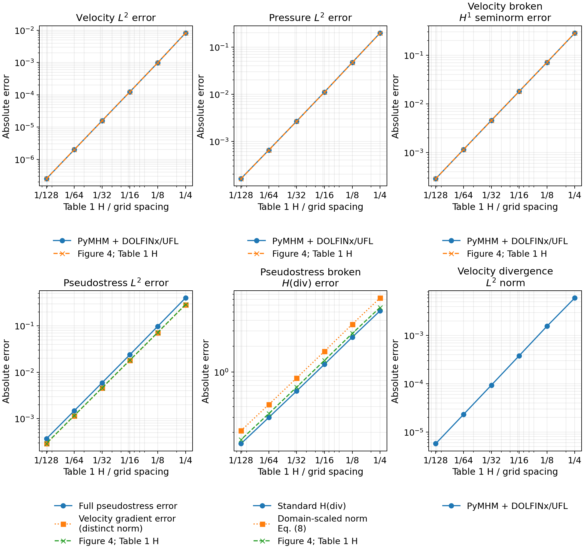
At \(n=16\), changing the complete discretization from P2/P2 with constant trace to P3/P3 with linear trace reduces the pressure L2 error from 0.615813 to 0.0110797. Both local and trace spaces change in that comparison; the reduction cannot be attributed to either one in isolation. Download P3/P3 results and comparison values.

Stress norms and published values

Equation (55) defines \(\sigma=-\nu\nabla u+pI\). At \(\nu=1\), its full Frobenius L2 error obeys the exact identity

\[ \|\sigma_h-\sigma\|^2 =\|\nabla e_u\|^2+2\|e_p\|^2-2(e_p,\nabla\!\cdot e_u), \qquad e_u=u_h-u,\quad e_p=p_h-p. \]

At \(n=4\), P2/P2 gives full stress error 5.69316, while the published stress L2 ordinate is approximately 3.53636. Direct quadrature gives \((e_p,\nabla\!\cdot e_u)=-0.00664421\) and an identity defect below \(4.6\times10^{-15}\). Cauchy–Schwarz bounds the full stress error between 5.68177 and 5.70220 using the measured pressure, gradient and divergence norms; 3.53636 lies outside that interval. The published ordinate is close to the velocity gradient error 3.53312. These bounds apply to the reconstructed fields in this comparison. The available MSL and mhm-mfem revisions do not supply the article's coefficient arrays or stress diagnostic; mhm-mfem also uses a different local formulation. The article's legend labels the ordinate stress L2 without specifying a deviatoric or gradient-only convention. The full-stress curve is therefore not reproduced under the stated definition. The plot reports the velocity gradient error as a separate quantity.

There is also a distinction between norm conventions. Equation (8) equips the conforming space H(div;Ω), used in the analysis, with a norm whose squared divergence term is weighted by the domain diameter squared:

\[ \|\sigma\|_{\operatorname{div},\Omega}^2 =\|\sigma\|_\Omega^2+d_\Omega^2\|\nabla\!\cdot\sigma\|_\Omega^2, \qquad d_\Omega=\sqrt2. \]

The numerical section instead names a broken H(div;T_H) norm, without explicitly repeating its weight. Figure 3 agrees with the standard broken H(div) norm, whose divergence weight is 1. The example reports and plots both weights. This is evidence for the diagnostic convention matching that curve, not a demonstrated contradiction between the conforming and broken norms. For P3/P3, neither weight reproduces the published stress curve within the extraction tolerance.

For P2/P2, the discrete pressure equation supplies a further consistency condition. Equation (47) gives zero mean divergence on every macroelement, so \(q_h=\nabla\cdot u_h\in P_1(T)\) is an admissible pressure test, including the pressure gauge. On the right isosceles triangles used here,

\[ \begin{aligned} \lVert\nabla q_h\rVert_T &\le \frac{\sqrt{72}}{h_T}\lVert q_h\rVert_T,\\ \lVert\nabla\cdot u_h\rVert &\le \frac{h_T\sqrt{72}}{768} \lVert\nabla\cdot(\sigma_h-\sigma)\rVert. \end{aligned} \]

The second inequality follows from equations (41)–(42), the first inverse inequality, \(\tau_T=m_T h_T^2/8\) and the admissible bound \(m_T\le1/96\). Let \(E_g,E_p,E_\sigma,E_d\) denote the four published gradient, pressure, stress L2 and stress H(div) errors. The stress identity and this pressure test then require both bounds

\[ \begin{aligned} \frac{\lvert E_g^2+2E_p^2-E_\sigma^2\rvert}{2E_p} &\le \lVert\nabla\cdot u_h\rVert,\\ \lVert\nabla\cdot u_h\rVert &\le \frac{h_T\sqrt{72}}{768} \sqrt{\frac{E_d^2-E_\sigma^2}{w}}, \qquad w\in\{1,2\}. \end{aligned} \]

Using \(h_T=1/n\) and the standard broken weight \(w=1\) gives:

n	Required divergence lower bound	USFEM divergence upper bound
4	3.14606	0.0334321
8	1.37141	0.00814188
16	0.616745	0.00200776
32	0.291128	0.000499449
64	0.143047	0.000124501

The intervals remain disjoint when every digitized ordinate varies independently by 1%; their smallest separation factor is 89.7. The domain weight \(w=2\) makes the upper bound smaller. Thus changing the admissible stabilization constant cannot reconcile all four ordinates under the stated geometry, spaces and stress conventions. This does not identify the historical connectivity or diagnostic. The Araya et al. (2016) uses the same full-stress definition. The consistency record preserves the assumptions, inverse constants, digitized inputs, interval calculation and source digests.

Orthogonal source projection has a definite effect on the divergence residual. Here \(d_h=\nabla\!\cdot\sigma_h\in P_2(T)^2\). For the orthogonal projection \(\Pi_2\),

\[ \|f-d_h\|_T^2=\|f-\Pi_2f\|_T^2+\|\Pi_2f-d_h\|_T^2. \]

Replacing \(f\) by \(\Pi_2f\), or by an orthogonal projection onto a larger polynomial space, reduces the divergence residual. It cannot explain a larger published H(div) error when the published stress L2 component is also smaller. Lower-degree projections or interpolation define other diagnostics; no such convention has been established for the historical calculation.

The exact forcing has degree five, so the squared divergence residual has degree ten; the degree-16 rule integrates this polynomial exactly. The article's diagnostic quadrature and coefficient arrays are unavailable, so the origin of the discrepancy is undetermined.

High-order numerical records

The complete numerical records are preserved in examples/results/stokes_2017_ufl_crisscross.json for P2/P2 and examples/results/stokes_2017_ufl_p3.json for P3/P3. examples/results/stokes_2017_ufl.json contains the diagonal-mesh comparison. All field samples are saved independently of plotting. Render the archived Darcy and Stokes comparisons with:

pixi run --locked -e notebooks python -m examples.plot_reproductions

The notebook 13_published_stokes_2017.ipynb presents the archived comparisons, the stress identity and both H(div) conventions without repeating FEM solves.

Stokes/Brinkman 2017: published conservation tables

For the Brinkman problem in Section 3.1.2, \(\nu=10^{-2}\), \(\gamma=1\), and

\[ u_1=y-\frac{1-e^{y/\nu}}{1-e^{1/\nu}},\qquad u_2=x-\frac{1-e^{x/\nu}}{1-e^{1/\nu}},\qquad p=x-y. \]

The source is \(-\nu\Delta u+u+\nabla p\), and exact velocity is prescribed. A numerically stable evaluation uses shifted exponentials, for example \((e^{(y-1)/\nu}-e^{-1/\nu})/(1-e^{-1/\nu})\) for the quotient. The Stokes calculations above do not cover the high-order Brinkman error curves for this boundary-layer problem.

Published mass-balance tables

The reported quantity is the unnormalized integrated defect \(\max_K|\int_K\nabla\cdot u_h\,dx|\), not a divergence L2 norm.

H in Table 1	Stokes, trace degree 0	Stokes, degree 1	Stokes, degree 2
1/4	5.056e-17	1.4801e-16	1.1266e-16
1/8	2.4720e-17	7.0998e-17	7.1869e-17
1/16	1.3487e-17	3.3093e-17	4.6540e-17
1/32	7.2352e-18	1.8744e-17	2.3442e-17
1/64	3.5950e-18	9.2944e-18	1.4982e-17
1/128	2.1444e-18	5.4785e-18	7.9874e-18

H in Table 2	Brinkman, degree 0	Brinkman, degree 1	Brinkman, degree 2	Monolithic USFEM P2/P2
1/4	7.7325e-16	9.3133e-16	1.1205e-15	1.8075e-2
1/8	5.8102e-16	1.3263e-15	1.4134e-15	5.5736e-3
1/16	8.5168e-16	1.1898e-15	9.2654e-16	1.1326e-3
1/32	1.0468e-15	1.2779e-15	1.3535e-15	1.4290e-4
1/64	1.2984e-15	1.3951e-15	1.2610e-15	1.3626e-5
1/128	1.2571e-15	1.2575e-15	1.3137e-15	1.1620e-6

These roundoff-scale MHM entries establish a conservation target; individual digits are not portable solver acceptance thresholds. The executed P2/P2 Stokes series has integrated macrocell defects from 1.46e-16 at n=4 to 4.82e-18 at n=128. P3/P3 gives 1.04e-16 to 3.59e-18 at n=4..128. These values confirm macrocell balance to solver precision, while the pointwise divergence L2 norms remain nonzero. Neither statement implies exactly divergence-free local fields.

Flux-reconstruction manuscript: Table 2

The author manuscript associated with Barrenechea et al. (2026) provides a further numerical table on printed page 23. These values are identified by manuscript version; identity with the final journal table has not been asserted.

The problem is \(u=\sin(2\pi x)\sin(2\pi y)\), \(A=I\), \(f=8\pi^2u\), homogeneous Dirichlet data on the unit square. Table 2 uses skeletal degree \(\ell=0\), continuous local degree \(k=2\), reconstruction degree \(m=2\), and fine diameter equal to half the macro diameter.

Printed macro diameter	Broken energy error	Estimator η	Effectivity
0.353	1.860	2.724	1.463
0.176	0.986	1.293	1.311
0.088	0.501	0.644	1.287
0.044	0.251	0.323	1.285
0.022	0.125	0.162	1.287

The energy norm is \(\|A^{1/2}\nabla(u-u_{Hh})\|_{L^2(\mathcal P)}\), and effectivity is \(\eta\) divided by that norm. The CSV retains the separate estimator components and printed rounding. The published moment reconstruction of equation (5.1) uses RT2; the native minimum-energy RT0 correction is a different construction and is not a reproduction of this table. Exact mesh connectivity, unrounded diameters and quadrature remain necessary inputs for a fully specified comparison.

References

• Christopher Harder, Diego Paredes, and Frédéric Valentin (2013). A family of Multiscale Hybrid-Mixed finite element methods for the Darcy equation with rough coefficients, Journal of Computational Physics 245, 107–130. DOI: 10.1016/j.jcp.2013.03.019.

• Rodolfo Araya, Christopher Harder, Abner H. Poza, and Frédéric Valentin (2017). Multiscale hybrid-mixed method for the Stokes and Brinkman equations—The method, Computer Methods in Applied Mechanics and Engineering 324, 29–53. DOI: 10.1016/j.cma.2017.05.027.

• Rodolfo Araya, Christopher Harder, Abner H. Poza, and Frédéric Valentin (2016). Multiscale hybrid-mixed method for the Stokes and Brinkman equations—The method. Universidad de Concepción, CI²MA, Preprint 2016-15. Institutional preprint. The journal publication is Computer Methods in Applied Mechanics and Engineering 324, 29–53 (2017), DOI: 10.1016/j.cma.2017.05.027.

• Gabriel R. Barrenechea, Larissa Martins, Weslley Pereira, and Frédéric Valentin (2026). An H(div; Ω)-Conforming Flux Reconstruction for the Multiscale Hybrid-Mixed Method, Multiscale Modeling & Simulation 24(2), 399–428. DOI: 10.1137/24M1673073.