Analytical Darcy lifts and source reconstruction

solve_darcy_analytic implements the lowest-order exact harmonic lifts of Harder, Paredes and Valentin (2013), §4.1 on affine triangles and tetrahedra. Each face carries a constant normal flux. The permeability is a constant symmetric positive-definite tensor in each local problem; the convenience solver uses one tensor throughout the domain.

Local space and source terms

For centroid \(c_T\), covariance \(C_T\), and dimension \(d\), use

\[ 1,\quad x_i-c_{T,i},\quad \frac12\big[(x-c_T)^T K_T^{-1}(x-c_T) -\operatorname{tr}(K_T^{-1}C_T)\big]. \]

The nonconstant basis functions have zero physical mean. Multiplication of their gradients by \(-K_T\) gives exactly the RT0 vector space. The harmonic responses therefore have exact polynomial normal traces, independently of the mesh used for the source response.

The complete pressure is \(p_h=p_0+p_\lambda+p_f\). The source lifting solves

\[ -\nabla\cdot(K_T\nabla p_f)=f-\Pi_0 f,\qquad K_T\nabla p_f\cdot n=0,\qquad \int_Tp_f=0. \]

It is zero for a constant source. For a variable source, continuous local Pk elements approximate this Neumann problem. The global load retains the full source moments against the exact harmonic lifts. In particular, the term \(-(f,p_\mu)\) in equation (42) is retained.

The classical RT0/P0 mixed method omits that load correction. Its RT0 field can also be integrated into a mean-preserving quadratic pressure using AnalyticDarcySpace.integrate_rt0; this operation preserves the classical pressure mean and does not supply the missing source correction. Section 4.1.1 expressly conditions its classical RT0 equivalence on neglecting that term.

Cosine problem: six resolutions

On the unit square, prescribe

\[ p=\cos(2\pi x)\cos(2\pi y),\quad f=8\pi^2p,\quad q=-\nabla p,\quad q\cdot n=0,\quad \int_\Omega p=0. \]

The grids have \(n=4,6,8,16,32,64\) subdivisions in each coordinate and \(2n^2\) macrotriangles, split on the lower-left to upper-right diagonal. Each source problem uses P2 on four subtriangles. Harmonic fields remain exact quadratics. Assembly uses Duffy order 10 and error integration order 12. The record also includes order 12/14 integration and source refinements 4 and 8 on the coarsest published grid.

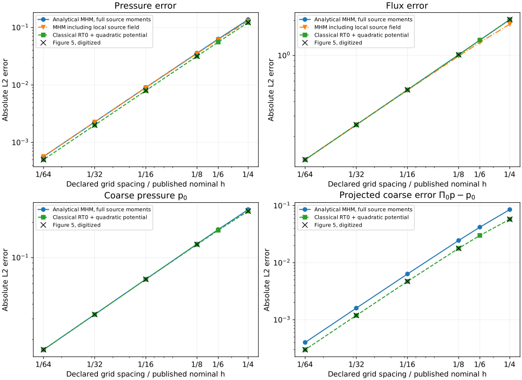
The two constructions produce the same trace-driven RT0 flux in this experiment, but different coarse pressures. At \(n=4\), the projected coarse pressure errors are 0.0852526 for analytical MHM and 0.0576301 for classical RT0; Figure 5 gives approximately 0.0576425. The quadratic pressure errors are 0.137703 and 0.122537, respectively, while the digitized value is 0.122294. Including the P2 source lifting changes the MHM pressure error to 0.130088. At \(n=64\), the complete pressure and flux errors are \(5.67681\times10^{-4}\) and 0.125872. At \(n=4\), increasing the source refinement from 4 to 8 changes the full pressure error from 0.130064 to 0.130051 and the full flux error from 1.85356 to 1.85299. Increasing both quadrature orders changes the six MHM error diagnostics by less than \(4\times10^{-15}\) relatively.

Thus the classical RT0 construction matches the plotted values, while the full-source analytical MHM implements equation (42). These are distinct discrete formulations for this nonconstant source. Matching the classical curve is not evidence that the full-source method or its full physical flux has reproduced Figure 5. The grid spacing \(1/n\) is also distinguished from the macro diameter \(\sqrt{2}/n\); the original connectivity is unspecified.

Independent checks

The automated checks use two- and three-dimensional anisotropic metric quadratic patches with both prescribed pressure and pure Neumann data. They verify the physical mean, every oriented face flux and the local basis means. A nonconstant polynomial source is compared against the complete P2 MHM assembly, including trace coefficients, retained means and reconstructed pressure. These tests check the source correction independently of any digitized figure.

Run the research campaign with:

pixi run --locked -e notebooks python -m examples.verify_analytic

The unrounded record is examples/results/analytic.json; notebook 43_analytical_darcy.ipynb presents the numerical comparison. The publication comparison retains the digitized data and the separately identified classical RT0 and primal P1 results.

References

• Christopher Harder, Diego Paredes, and Frédéric Valentin (2013). A family of Multiscale Hybrid-Mixed finite element methods for the Darcy equation with rough coefficients, Journal of Computational Physics 245, 107–130. DOI: 10.1016/j.jcp.2013.03.019.