Darcy flow and heterogeneous media

These cases compare the native primal P1 and mixed RT0/P0 local formulations against analytical pressure and physical Darcy flux. They also distinguish conservation of the skeleton unknown from conservation of the reconstructed field. All problems use

\[ q=-K\nabla p,\qquad \nabla\cdot q=f \]

on the unit square, with analytical pressure prescribed on its entire boundary. Harder, Paredes and Valentin (2013) give the original primal formulation; verification reports additional refinement levels.

Both local formulations and the flux reconstruction on this page are executed by pyMHM's native NumPy/SciPy backend. Their reference fields are analytical expressions. The separate DOLFINx assembly verification, MSL primal comparison, and NeoPZ mixed comparison identify the external implementations used for additional checks.

Smooth pressure: compare both local formulations

For unit permeability, choose

\[ \begin{aligned} p(x,y)&=\cos(\pi x)\cos(\pi y),\\ q(x,y)&=\pi\bigl(\sin(\pi x)\cos(\pi y), \cos(\pi x)\sin(\pi y)\bigr),\\ f(x,y)&=2\pi^2\cos(\pi x)\cos(\pi y). \end{aligned} \]

This analytical problem appears in Durán et al. (2019). The present triangular discretization and local spaces differ from the paper's numerical experiments; the figures verify the specified problem rather than reproduce its tables.

The coarse discretization uses a 4 × 4 macro square grid split into 32 macro triangles, four subdivisions along each local edge, and 512 fine triangles. The normal-flux trace is constant on each macroface. Both formulations use the same meshes, boundary data and quadrature: Duffy order 6 for assembly and order 8 for independent error integration.

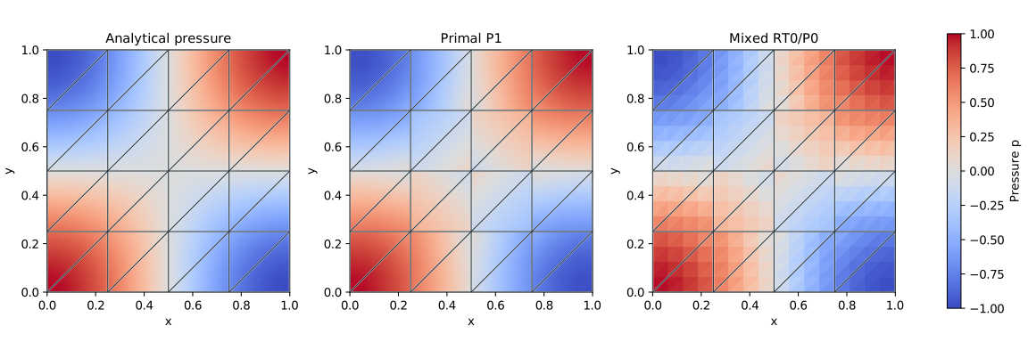
Pressure

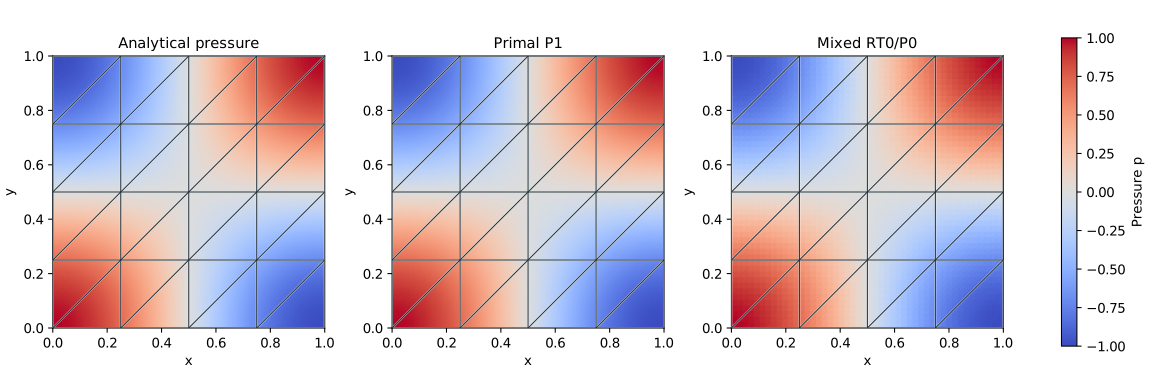
The analytical solution has alternating positive and negative corner regions and vanishes on the two midlines. All three panels use the same pressure scale. The primal pressure is piecewise linear inside each macrocell; the mixed pressure is piecewise constant on fine triangles. Broken macro traces remain separate when plotting, and P0 pressure is not interpolated into a smooth field.

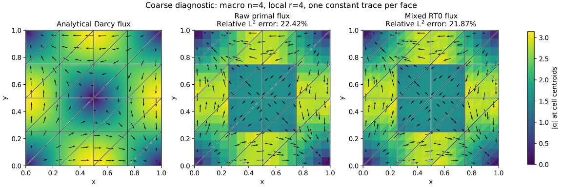
Physical flux on the coarse mesh

The relative L2 flux errors are 22.42% (primal) and 21.87% (mixed). The visible mosaic includes a substantial approximation error. A small solver residual and a conservative RT0 field do not establish a sufficiently resolved solution. The independent accuracy study quantifies the separate effects of macro, local and trace refinement. The matched coarse-case reference computations compare this specific discretization with MSL and NeoPZ, using the same nonzero weak Dirichlet pressure data.

The vector field is directed down the pressure gradient. Colors show its magnitude, while arrows show its direction and relative size using the same arrow scale in all panels. Numerical magnitudes and arrows are evaluated at fine-cell centroids; the analytical panel is sampled independently. In particular, the centroid display does not show the full affine variation of an RT0 field inside a triangle.

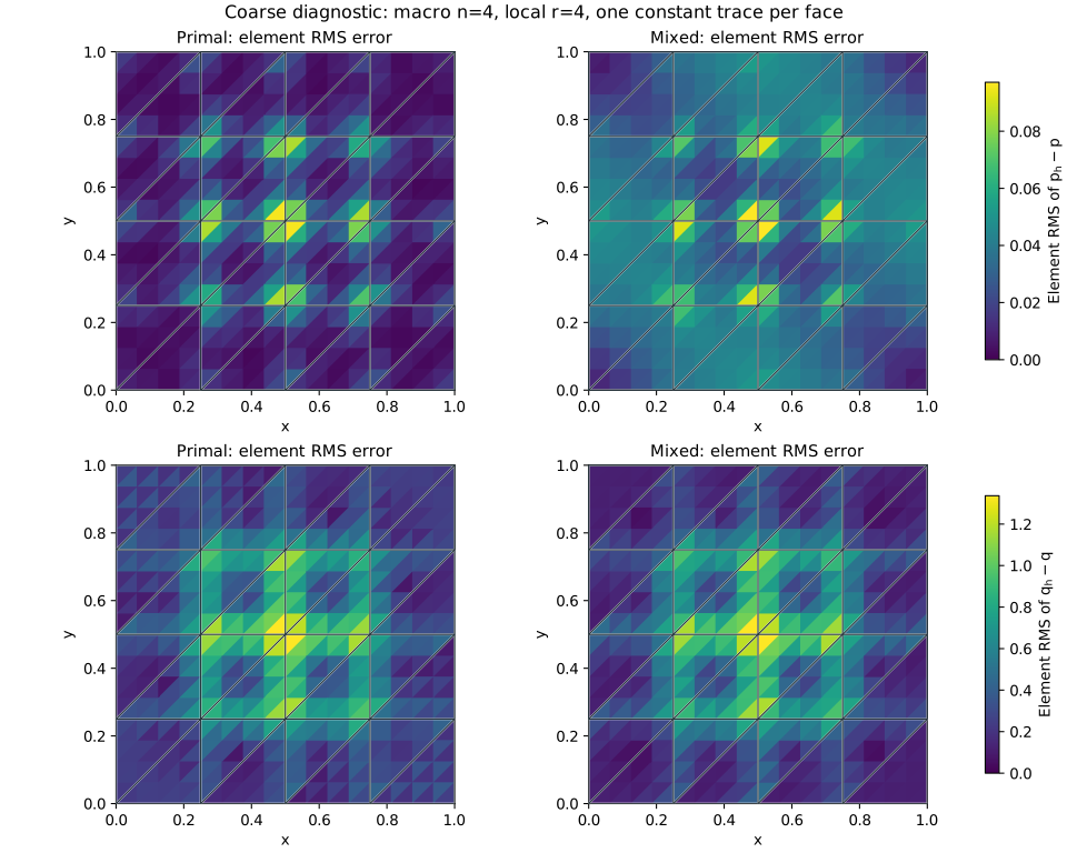
Error location and integrated norms

Each map shows an element root-mean-square error,

\[ e_T(v)=\left(\frac{1}{|T|}\int_T |v_h-v|^2\,dx\right)^{1/2}. \]

The pressure panels share a color scale, and the flux panels share another. These are errors integrated over each element, rather than errors sampled only at nodes or centroids. The global norm satisfies \(\|v_h-v\|_{L^2(\Omega)}^2=\sum_T |T|e_T(v)^2\).

Local formulation	Pressure L2 error	Physical flux L2 error
Primal P1	2.457274e-2	4.979959e-1
Mixed RT0/P0	4.034965e-2	4.857458e-1

The smaller P1 pressure error must be interpreted together with its richer pressure space. The mixed formulation has a slightly smaller flux error in this run. A single grid does not establish a convergence rate or a general ordering between the two formulations.

An enriched computation

Retain the same 32 macrotriangles and problem data, refine each local edge into 12 parts, and divide each macroface into six constant trace segments. This gives 4608 fine triangles and reduces the relative physical flux error to 3.28% for primal P1 and 2.22% for mixed RT0. The plot keeps the numerical fields unsmoothed, with identical scales within each comparison.

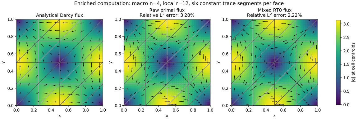
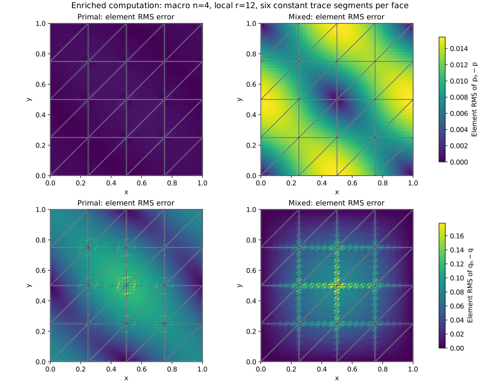
The improvement requires enriching the trace. Refining only the local triangles leaves a flux-error plateau near 22%. Five-point macro, local and trace studies, normal-jump diagnostics, and independent DOLFINx/UFL checks are reported in the Darcy flux verification study. The separate published-result comparisons distinguish analytical verification from reproduction of an article's actual error curves.

Permeability contrast of 1000

A fitted vertical interface separates two constant permeabilities:

\[ K(x)=\begin{cases}1,&x<1/2,\\1000,&x>1/2,\end{cases} \qquad p(x)=\begin{cases}1-x,&x\leq1/2,\\ \frac12-\frac{x-1/2}{1000},&x>1/2. \end{cases} \]

Pressure is continuous, its slope changes by a factor of 1000, and the exact physical flux is \(q=(1,0)\) everywhere. Thus \(f=0\), including across the interface in the distributional sense. Exact pressure is prescribed on all four sides, using Dirichlet data also on the top and bottom boundaries.

The material interface coincides with macro and fine edges. P1 can represent the piecewise affine pressure exactly, and RT0 can represent its constant flux. The mixed P0 pressure retains its expected cell-average representation error.

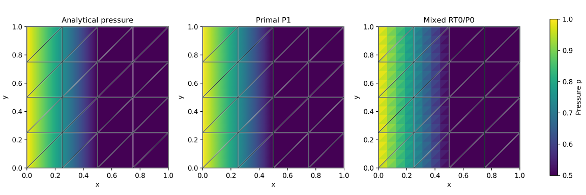
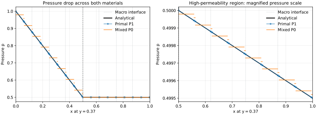
The right-hand pressure drop is only \(5\times10^{-4}\), so a second profile panel magnifies this scale. The profile at \(y=0.37\) shows each P0 segment with its own endpoint limits, without interpolating across jumps. Primal P1 segments coincide with the analytical curve to plotting precision.

Local formulation	Pressure L2 error	Physical flux L2 error
Primal P1	1.130122e-16	5.278423e-13
Mixed RT0/P0	1.041667e-2	4.159053e-13

For this diagonal triangular grid with fine spacing \(h=1/(4\cdot4)=1/16\), the analytical P0 projection error is

\[ \|p-\Pi_0p\|_{L^2(\Omega)} =\frac{h}{6}\sqrt{1+10^{-6}} =1.0416671875\times10^{-2}. \]

It agrees with the computed mixed pressure error. The plotting script checks this agreement numerically. The remaining primal pressure and both flux errors are at floating-point accuracy for this fitted problem; they are not reported as exact zeros. This case does not test cut-cell integration, arbitrary coefficient contrast, or robustness on unfitted meshes.

Conservation: skeleton, raw gradient and recovered field

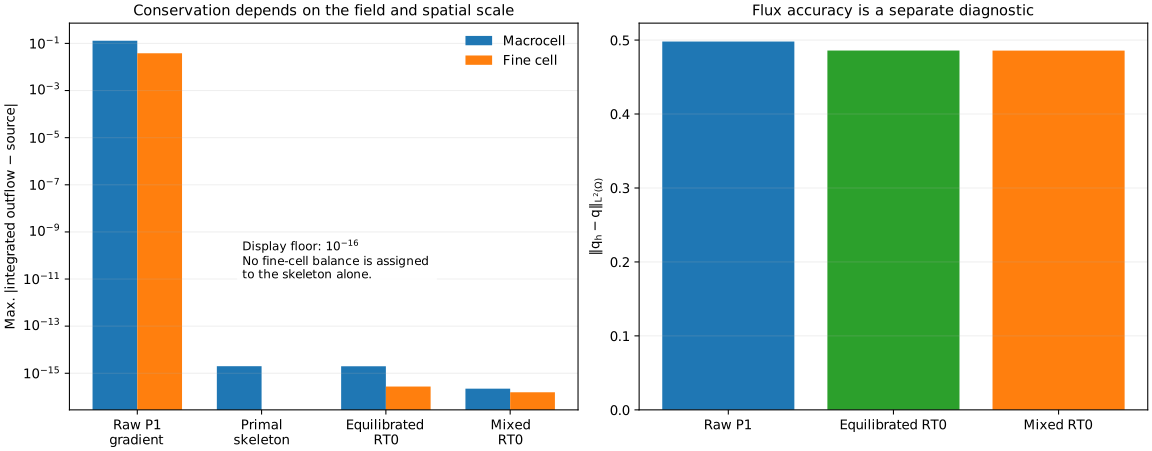
Return to the cosine problem, whose source is nonzero. The raw primal flux \(-\nabla p_h\) is constant on each fine triangle, so its fine-cell divergence is zero there. It cannot balance a nonzero cell source, even though the MHM skeleton satisfies the macrocell balance equations.

equilibrate_flux reconstructs an RT0 field by a constrained minimum-energy correction, matching the prescribed skeleton normal flux and the assembled source integral on each fine cell. The separately solved pyMHM mixed problem instead constructs its RT0 flux as a primary unknown. These are different procedures.

The plotted defect on a cell \(T\) is

\[ d_T=\int_{\partial T}q_h\cdot n_T\,ds-\int_T f\,dx. \]

Macrocell and fine-cell bars report \(\max_T|d_T|\) on their respective partitions. Source integrals use assembly quadrature, so the diagnostic measures the discrete balance equations. A skeleton alone has no fine-interior flux field; consequently, its fine-cell defect is left unspecified.

Field or trace	Maximum macrocell defect	Maximum fine-cell defect
Raw primal gradient	1.304109e-1	3.830590e-2
Primal skeleton	2.220446e-16	Not defined
Equilibrated RT0 field	2.402592e-16	1.977585e-16
Mixed RT0 field	1.665335e-16	1.370432e-16

The logarithmic chart uses a display floor of \(10^{-16}\); unmodified values are retained in the metrics file. Conservative fields still have approximation error: the recovered flux has L2 error 0.4858182, compared with 0.4979959 for the raw primal gradient and 0.4857458 for the mixed flux.

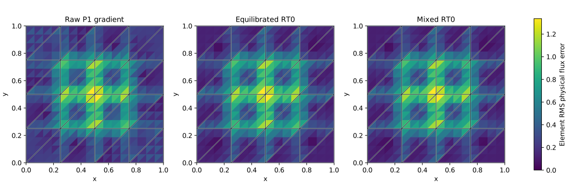
The modest improvement in this case is an observation, not a guarantee that every conservative reconstruction reduces the L2 error. This minimum-energy RT0 correction is also distinct from the higher-order moment construction discussed in the literature catalogue.

Reproduce and export

From the repository checkout, run:

pixi run --locked -e notebooks python -m examples.plot_darcy_cases

The script limits numerical thread pools to one thread and writes ten SVG figures, ten PNG figures and machine-readable metrics. Use --macro-resolution, --local-refinement and --output-directory to generate another experiment. Macro resolution must be even so that the material interface remains fitted. Changing these parameters changes the measured values; the tables above describe the default run. The enriched comparison keeps r=12,s=6 while using the requested macro resolution.

The analytical panels use a separate display grid. Error maps and norms use quadrature on the actual finite elements. The SVG and PNG files share the same computed data and are suitable for inspection or export.

References

• Omar Durán, Philippe R. B. Devloo, Sônia M. Gomes, and Frédéric Valentin (2019). A multiscale hybrid method for Darcy’s problems using mixed finite element local solvers, Computer Methods in Applied Mechanics and Engineering 354, 213–244. DOI: 10.1016/j.cma.2019.05.013.