Coarse cosine flux: matched reference computations

This comparison uses exactly the coarse discretization in the Darcy gallery: 32 macrotriangles, 512 fine triangles, and one constant normal-flux trace per macroface. It checks complete physical fields, rather than comparing only error norms or visual similarity.

Problem and discrete spaces

On the unit square, with unit permeability,

\[ p=\cos(\pi x)\cos(\pi y),\qquad \boldsymbol q=\pi\begin{pmatrix} \sin(\pi x)\cos(\pi y)\\ \cos(\pi x)\sin(\pi y) \end{pmatrix},\qquad f=2\pi^2p. \]

The boundary pressure is the restriction of this nonzero analytical pressure. It is imposed weakly through the global skeleton.

Parameter	Value
Macro mesh	Four squares per axis; each split along its lower-left to upper-right diagonal
Local mesh	Four subdivisions per macroedge; 16 fine triangles per macrotriangle
Primal local space	Continuous P1 pressure inside each macrotriangle
Mixed local spaces	RT0 flux and P0 pressure on each fine triangle
Skeleton	One unsplit P0 segment per macroedge, including boundary edges
pyMHM quadrature	Duffy order 6 for assembly; order 8 for analytical errors; Gauss 5 for boundary moments
Error normalization	\(\lVert q\rVert_{L^2}=\pi/\sqrt{2}\) and \(\lVert p\rVert_{L^2}=1/2\)

The separate MSL sine comparison uses crisscross macrotriangles, P1 traces, a different local refinement, and homogeneous boundary data. Its agreement does not establish agreement for this case.

Primal comparison with MSL

The reference uses msl_mhm, msl_cg, and msl_core at the revisions listed in the MSL provenance. Its comparison adapter assembles the weak boundary functional \(\int_{\partial\Omega}g\,\psi_i\,ds\) using MSL's signed trace orientation and native boundary quadrature. MSL supplies the local operators, global matrix, spaces, and solve sequence. The boundary assembly is shared by the cosine and sine comparison drivers.

Zero, constant, and affine pressure patches check this boundary assembly. All have \(f=0\); the affine pressure is \(p=1+x+2y\), with flux \((-1,-2)\). Numerical values, expression strings, and Lua callbacks are read from the problem data and evaluated through the same adapter.

Pressure	Trace degree / segments per face	Local subdivisions	MSL pressure L2 error	MSL flux L2 error
Zero	P0 / 1	4	0	0
Constant 1	P0 / 1	4	1.67e-16	3.07e-15
Affine	P1 / 1	4	1.07e-15	1.89e-14
Affine	P1 / 2	8	1.20e-15	3.83e-14

For the cosine boundary data, MSL reproduces the coarse primal field, including its visible macrocell structure:

Quantity	MSL primal P1	pyMHM primal P1
Pressure L2 error	0.0245727421091423	0.0245727421091422
Raw flux L2 error	0.497995938749214	0.497995938749214
Relative flux L2 error	22.41769345%	22.41769345%

All 480 broken pressure nodes and 512 fine triangles were matched by physical coordinates. Exact P1 mass integration gives a pressure difference of \(9.39\times10^{-16}\) in L2. Exact P0 vector integration gives a raw flux difference of \(7.98\times10^{-15}\). Maximum differences are \(2.55\times10^{-15}\) at pressure nodes and \(1.78\times10^{-14}\) in flux components. No averaging across macrofaces enters the comparison.

The MSL forcing parameter is 8, requesting native integration degree 9; its explicit boundary integration requests degree 8, giving five Gauss points as in pyMHM. These integer parameters are not the same as a Duffy tensor-product order. Analytical errors in the table are independently reintegrated using Duffy order 8 on the exported fields.

Mixed comparison with NeoPZ

The mixed reference uses native NeoPZ RT0/P0 assembly at revision 4c6b6d2, with EHDivConstant order zero. The native operator is restricted to one constant normal-flux trace per macroface using \(T^{\mathsf T}AT\); the restricted system is solved with SciPy, and the physical fields are reconstructed by NeoPZ. This is separate from execution of an MSL mixed solver or NeoPZ's historical MHM controller. The NeoPZ comparison defines the spaces and the restriction in detail.

Quantity	NeoPZ restricted RT0	pyMHM mixed RT0
Pressure L2 error	0.04034964721748132	0.04034964721748275
Flux L2 error	0.4857458152980587	0.4857458152980586
Relative flux L2 error	21.86624415%	21.86624415%

The full-field L2 differences are \(1.46\times10^{-14}\) in pressure, \(6.94\times10^{-14}\) in flux, and \(3.49\times10^{-14}\) in divergence. The relative residual of the restricted native system is \(3.69\times10^{-15}\). Recomputed fine- and macrocell integrated conservation defects are below \(5.5\times10^{-16}\) in both implementations.

The spatial figure evaluates the retained restricted coefficient vector through NeoPZ's native EHDivConstant field evaluator and compares it with a current PyMHM solve of the same 32-macrotriangle, 512-fine-triangle problem. Pressure remains P0 on each fine cell; signed RT0 components are rendered affinely inside each cell, with independent one-sided values across interfaces. Every panel outlines the actual macro mesh. Error norms use quadrature rather than display samples.

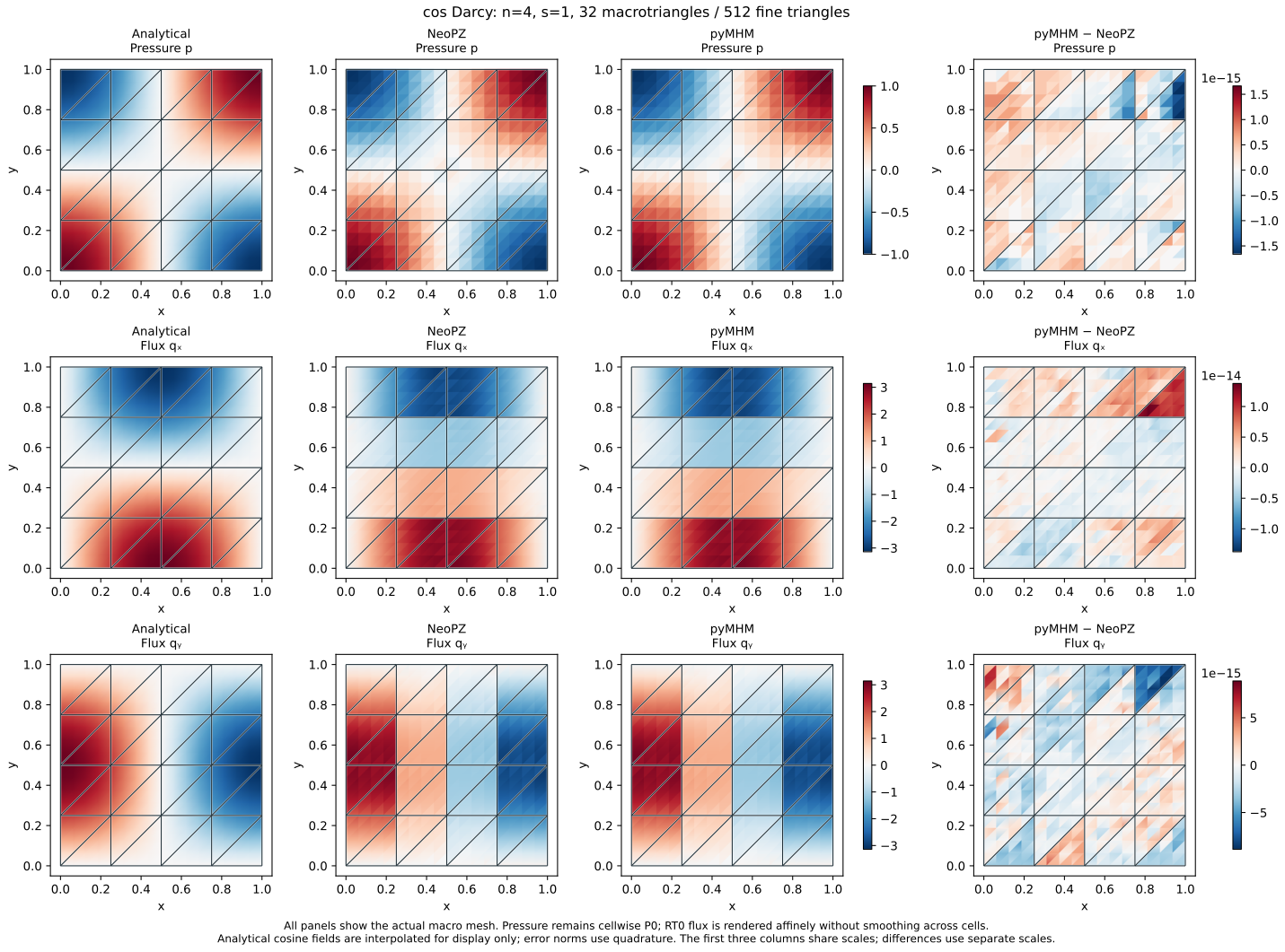
Independent integration at Duffy orders 8 and 10 recovers the retained NeoPZ pressure and flux errors to rounding accuracy. In this replay, the current PyMHM/NeoPZ L2 field differences are \(3.58\times10^{-16}\) in pressure, \(3.53\times10^{-15}\) in flux and \(3.77\times10^{-14}\) in divergence. Fine-cell integrated conservation defects are below \(3.5\times10^{-16}\). The replay receipt records the retained coefficient digest, the native evaluator digest and the new paired field archive digest separately. Native evaluation does not assemble or solve the reference system again, so its algebraic residual is not remeasured; the restricted residual above belongs to the original executed comparison.

Native NeoPZ uses volume integration order 12 and boundary Gauss order 20 (11 points). Increasing pyMHM's volume quadrature from 6 to 10 changes the flux by only \(1.56\times10^{-15}\) in L2. The coarse flux error is not explained by insufficient volume quadrature in this test.

What the coarse pattern demonstrates

A constant trace on an entire macroface supplies very limited interface resolution. In the mixed method, the reconstructed normal flux is constrained to be constant there. For the primal method, this is the Neumann trace used in the local solves; the raw gradient is not itself an H(div) field and need not coincide pointwise with that trace.

The shared MSL adapter also verifies the following primal spaces against pyMHM. The first three rows use identical macro and fine meshes; only the trace space changes. The final row refines both the local mesh and the trace.

Trace degree	Segments per macroface	Fine triangles	Relative flux L2 error, both codes	Flux field difference in L2
P0	1	512	22.41769345%	7.98e-15
P0	2	512	10.10440143%	7.79e-15
P1	1	512	9.77863384%	8.12e-15
P1	2	2048	4.89687669%	1.62e-14

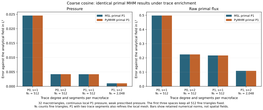
This norm plot uses the original MSL/PyMHM measurements, with their rendering provenance. It does not substitute newly generated fields for the original MSL coefficient snapshots, which are not distributed with this checkout.

Keep both meshes fixed and enrich only the mixed trace to four P0 segments per macroface. The relative flux error drops from 21.8662% to 5.6697%. The enriched pyMHM and NeoPZ fluxes still agree to \(2.32\times10^{-14}\) in L2. This controlled experiment separates trace resolution from local refinement. The five-point refinement studies examine both separately.

These comparisons establish agreement for the specified discrete problems. The approximately 22% flux error remains substantial: agreement between codes and conservation do not make this coarse discretization an accurate reference solution. The mixed spatial figure preserves the one-sided numerical fields without smoothing.

Archived evidence

The comparison summary, primal report and mixed report retain full precision measurements and the checksums of the original acquisition. The primal report records eight boundary and trace-space checks and the shared MSL adapter digests. Those original MSL coefficient snapshots are not distributed.

The downloadable mixed physical-field replay and receipt accompany the spatial figure above. The NPZ contains exact triangle connectivity, macro geometry, cellwise P0 pressure and three declared barycentric RT0 samples for both implementations. These samples determine the physical affine vector in each fine cell, without reconstructing an unspecified algebraic basis or averaging across interfaces. It is a separately identified replay archive, not a replacement for an original acquisition file with a different digest.

examples.plot_neopz_comparison.plot_fields reads this replay through its recorded checksum and renders it without invoking either solver. The complete historical examples.plot_reference_comparison command additionally requires the original MSL field archives.