Stokes, Brinkman, and Oseen: exact fields and computed solutions

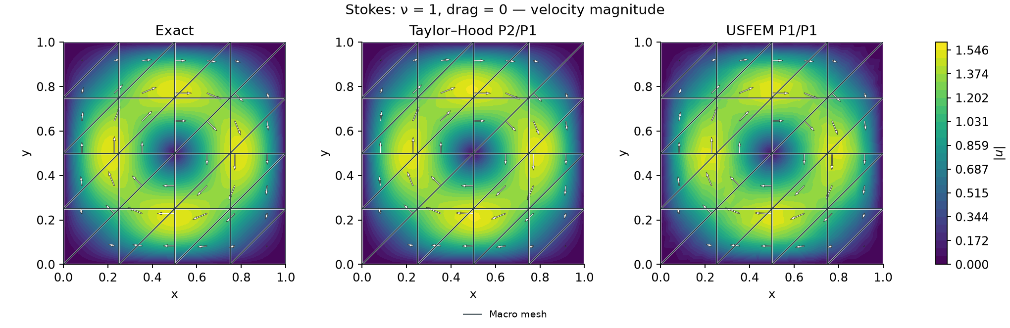
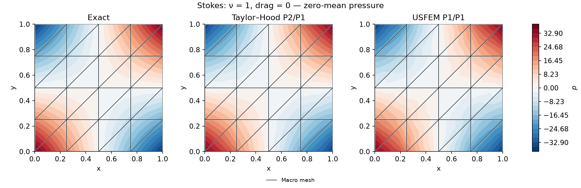
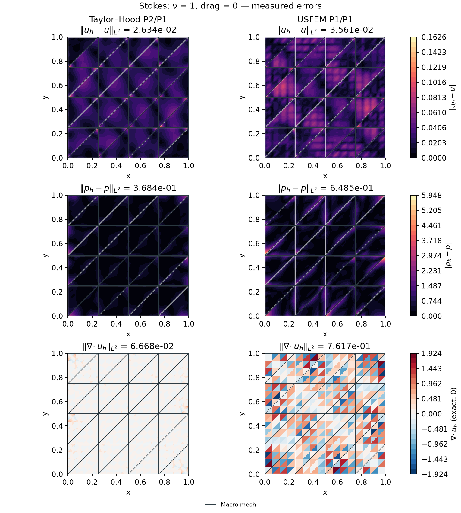
These examples compare reconstructed MHM fields with an analytical solution on \(\Omega=(0,1)^2\). They expose errors that a small algebraic residual cannot measure: velocity approximation, pressure approximation, and pointwise incompressibility. Every exact/numerical field comparison uses one color scale; error and divergence panels use one scale per row across the methods.

The Stokes data are the polynomial problem in §3.1.1 of Araya et al. (2017). The Brinkman and Oseen cases below use the same fields with forcing derived for each operator. They verify these operators against a known solution; the meshes and local spaces do not reproduce a published convergence table or the paper's boundary-layer examples. These figures are generated by pyMHM's native NumPy/SciPy implementation; their reference is the analytical polynomial field, not an MSL or MFEM calculation. Independent DOLFINx/UFL assemblies appear in the pressure convergence study.

Equations and independent reference

Write \(a(s)=s^2(s-1)^2\) and define

\[ \psi=-128a(x)a(y),\qquad u=\begin{pmatrix}\partial_y\psi\\-\partial_x\psi\end{pmatrix}, \qquad p=150(x-\tfrac12)(y-\tfrac12). \]

The symbol \(u\) denotes velocity; \(\nu\) below denotes viscosity. This reference has \(\nabla\cdot u=0\), vanishes on the boundary, and satisfies \(\int_\Omega p=0\). For each coefficient choice, the force is obtained by analytical polynomial differentiation:

\[ f=-\nu\Delta u+\gamma u+(\beta\cdot\nabla)u+\nabla p. \]

examples/manufactured.py provides the Stokes/Brinkman terms; examples/plot_flow_cases.py evaluates the additional Oseen derivative. Both local methods use the pseudostress operator \(-\nu\Delta u\), with a single global mean-pressure constraint. Araya et al. (2017) give this formulation; the UFL guide shows how to declare the volume operator and boundary pairing.

The displayed run uses a \(4\times4\) diagonal macro grid: 32 macrotriangles, four subdivisions per local edge, 512 microtriangles, and degree-one, two-component skeleton spaces. Local velocity/pressure spaces are P2/P1 for Taylor–Hood and residual-stabilized P1/P1 for USFEM. Assembly uses Duffy quadrature order 6; velocity and pressure errors use order 8. The higher assembly order exactly integrates the degree-nine Taylor–Hood load product when Brinkman drag is present. The USFEM force includes the complete drag-dependent residual terms.

Case	Local method	\(\lVert u_h-u\rVert_{L^2}\)	\(\lVert p_h-p\rVert_{L^2}\)	\(\lVert \nabla\cdot u_h\rVert_{L^2}\)
Stokes, \(\nu=1\)	Taylor–Hood	2.6339e-2	3.6839e-1	6.6679e-2
Stokes, \(\nu=1\)	USFEM	3.5607e-2	6.4850e-1	7.6174e-1
Brinkman, \(\nu=1,\gamma=100\)	Taylor–Hood	2.1117e-2	3.9875e-1	6.5101e-2
Brinkman, \(\nu=1,\gamma=100\)	USFEM	3.0244e-2	6.6913e-1	7.6847e-1
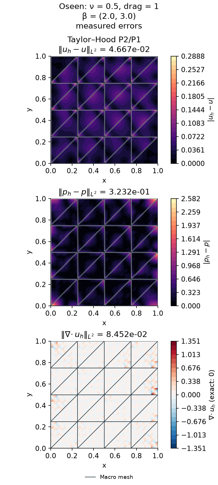
Oseen, \(\nu=0.5,\gamma=1,\beta=(2,3)\)	Taylor–Hood	4.6673e-2	3.2324e-1	8.4522e-2

The recorded algebraic residuals are below \(10^{-15}\), while the approximation errors are substantially larger. The complete values and run parameters are available in the JSON record. The figure record identifies the spatial plots and verifies the original physical norms within \(5\times10^{-14}\) relatively.

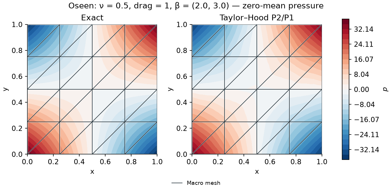
The coarse pressure fields below have measurable interface jumps. See the pressure convergence study for independent assembly checks, five-level refinement, separate local/trace studies, and profiles preserving both interface limits. A refined Taylor–Hood case reaches 0.0398% relative pressure error; localized pressure errors remain visible in the low-order USFEM case.

Polynomial Stokes problem

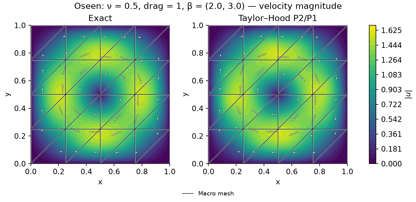
The velocity forms a smooth recirculation with zero boundary values. The pressure is a zero-mean bilinear saddle. Both methods recover these structures on the same macro and micro grids.

Exact, Taylor–Hood, and USFEM Stokes velocity magnitudes on a common scale

Exact and numerical zero-mean Stokes pressures on a common symmetric scale

The following rows show velocity error magnitude, pressure error magnitude, and signed discrete divergence. The exact divergence is zero. On this mesh, USFEM has a substantially larger divergence norm despite comparable velocity error; weak incompressibility does not imply pointwise divergence-free reconstruction. No equivalence of the methods' local degrees of freedom is assumed.

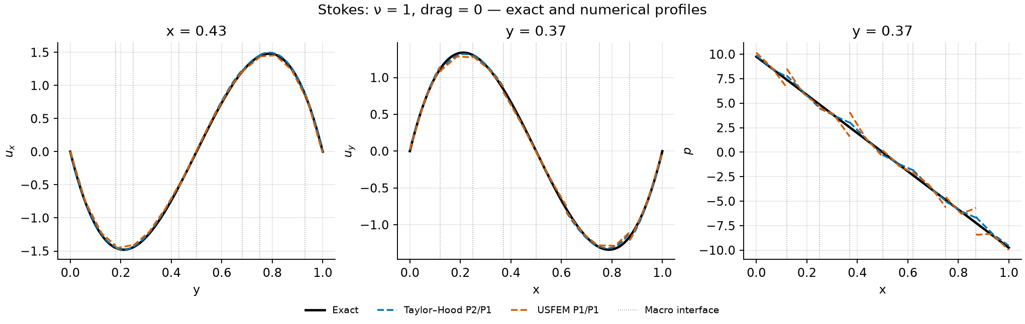
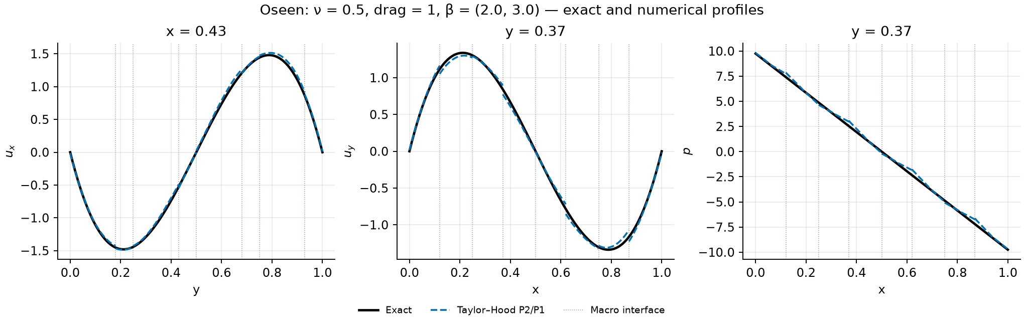
Stokes velocity and pressure errors and divergence, with integrated norms in the titles

Profiles sample the actual P1/P2 finite element polynomials. They cross the macro skeleton and therefore retain any local-field jumps. The lines \(x=0.43\) and \(y=0.37\) avoid alignment with complete macro edges. Each crossed macrocell is drawn as an independent segment, retaining both one-sided values at an interface; dotted lines mark those intersections.

Stokes velocity components and pressure profiles against the analytical curves

The verification results also report coarse-grid refinement. A single field plot does not establish an asymptotic convergence rate.

Brinkman with positive drag

Here \(\nu=1\), \(\gamma=100\), and \(\beta=0\). The force contains \(100u\), so the exact velocity and pressure remain those of the Stokes case. The forcing varies consistently with drag in this manufactured family; the experiment measures approximation error for the same exact fields.

Exact and computed Brinkman velocity magnitudes for drag 100

Exact and computed Brinkman pressures for drag 100

Brinkman velocity and pressure errors and signed divergence

Brinkman velocity and pressure cross sections compared with exact curves

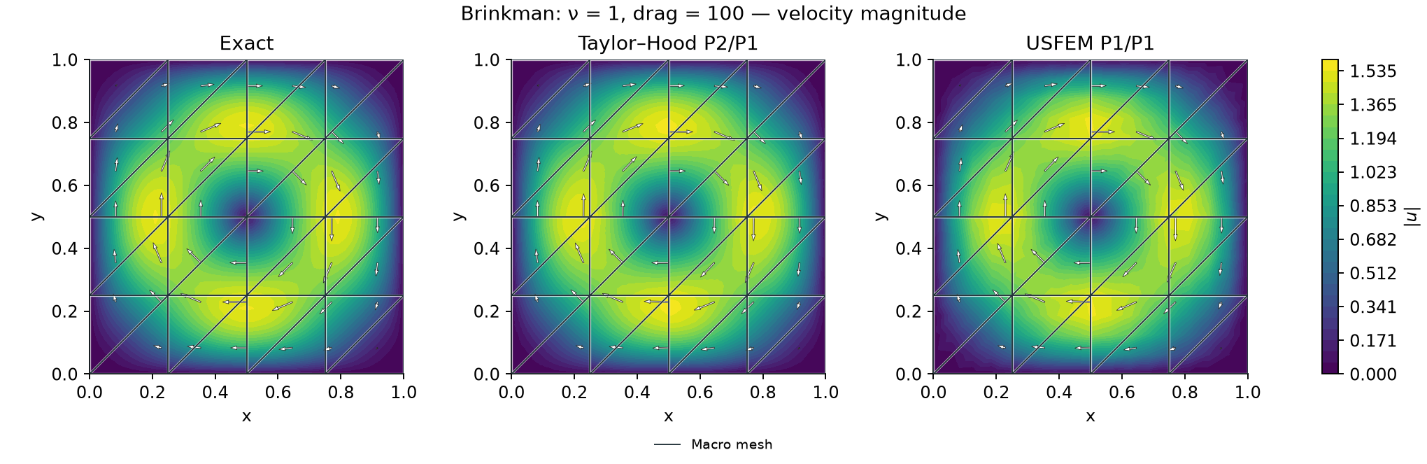
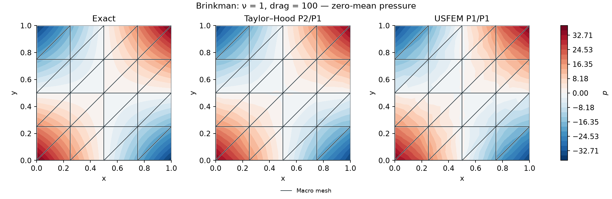
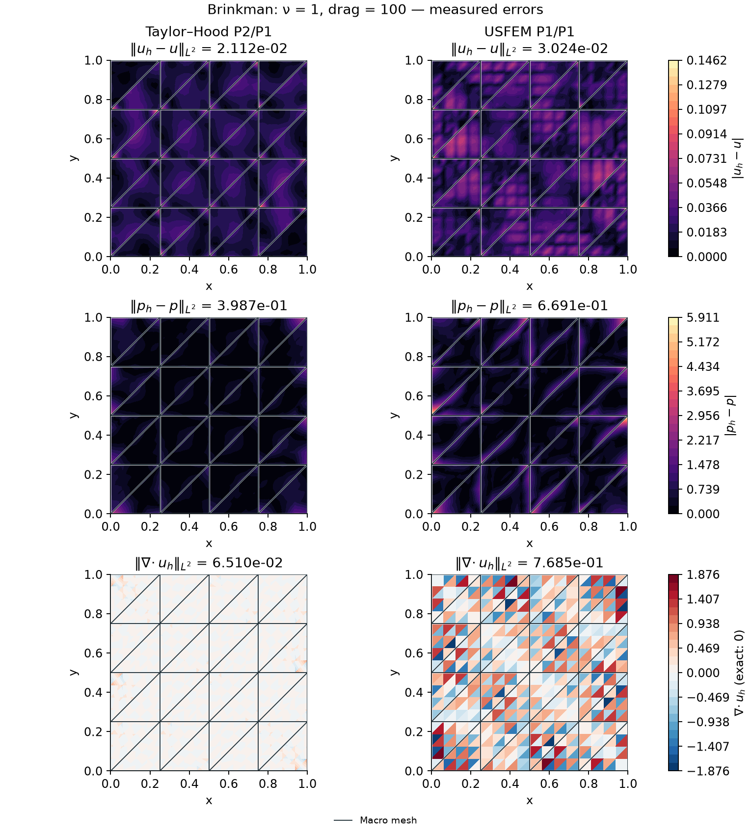
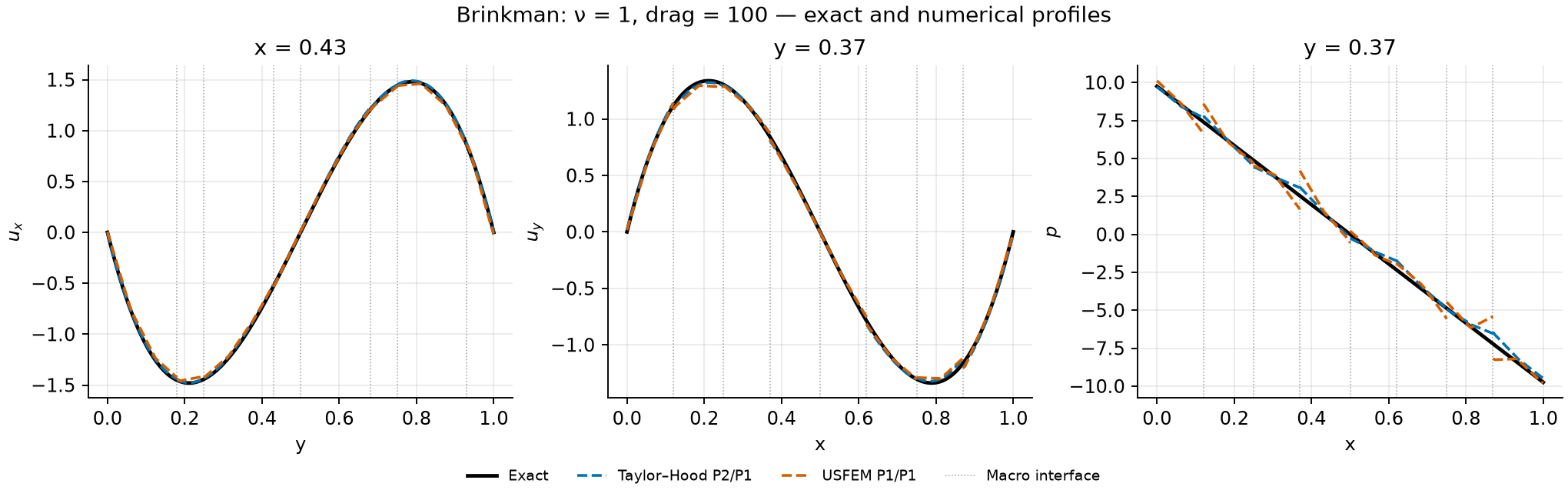
The errors in this smooth manufactured problem remain comparable to the zero-drag run. This observation does not establish robustness as viscosity tends to zero, accuracy in unresolved Brinkman layers, or stability for tensor-valued heterogeneous drag. Those require separate coefficient and mesh studies.

Oseen with constant background transport

Use \(\nu=0.5\), \(\gamma=1\), and \(\beta=(2,3)\). The additional force \((\beta\cdot\nabla)u\) is differentiated analytically. The native Oseen method uses Taylor–Hood locals, skew advection, and its corresponding Robin pseudotraction in this example. The separate formulation="oseen" path implements the equal-order stabilized method, including variable convection and its full residual; see the adaptive Oseen cases.

Exact and Taylor–Hood Oseen velocity magnitudes on a common scale

Exact and Taylor–Hood Oseen pressure on a common scale

Oseen velocity and pressure errors and divergence against the analytical reference

Oseen velocity and pressure profiles with analytical reference curves

An additional affine consistency check uses \(u=(y,-x)\), \(p=0\), \(\gamma=1\), and the same \(\beta\). Its force is \(f=u+(3,-2)\). Measured errors are \(7.51\times10^{-15}\) in velocity, \(2.13\times10^{-13}\) in pressure, and \(5.12\times10^{-14}\) in divergence. The exactly representable patch also verifies the field evaluator and transport signs. The example covers smooth linear Oseen flow; adaptive error estimation, convection-dominated layers and nonlinear Navier–Stokes flow are outside its scope.

Reproduce and interpret the figures

From the repository root:

pixi run --locked -e notebooks python -m examples.plot_flow_cases

The script writes 12 SVG figures, 12 matching PNG files, and metrics.json to docs/figures/flow/. It runs with one native numerical thread. Optional --macro-resolution, --local-refinement, and --output arguments support independent mesh studies without editing the script. The documented numbers refer to the default run; changing these arguments changes the experiment.

Color plots evaluate the local polynomials on three rendering subdivisions per microtriangle, then interpolate colors within the rendering triangles. They preserve independent values on opposite sides of a macro interface. Pointwise color extrema are sampled values, not integrated error norms or certified maxima. The table and plot-title norms come from finite element quadrature on the original microtriangles. Arrows use sampled velocity vectors and the same length scale in exact and numerical panels. Profiles evaluate the local polynomials directly.

Notebooks 05_stokes_published_problem.ipynb and 06_brinkman_and_oseen.ipynb provide shorter interactive versions of the analytical problem and consistency checks; see the notebook guide.

References

Rodolfo Araya, Christopher Harder, Abner H. Poza, and Frédéric Valentin (2017). Multiscale hybrid-mixed method for the Stokes and Brinkman equations—The method, Computer Methods in Applied Mechanics and Engineering 324, 29–53. DOI: 10.1016/j.cma.2017.05.027.