Stokes pressure: assembly checks, interface jumps, and refinement

The polynomial Stokes problem exposes a limitation of the low-order local approximation: a visually plausible velocity can coexist with an inaccurate, discontinuous pressure. The coarse P1/P1 pressure has localized errors and interface jumps in its finite element coefficients, measured below in the zero-mean pressure gauge.

This study uses the analytical data of Araya et al. (2017), §3.1.1, with viscosity one, zero drag, homogeneous velocity boundary data, and zero mean pressure. The exact pressure is \(p=150(x-1/2)(y-1/2)\), with \(\|p\|_{L^2}=12.5\). The velocity is derived from the streamfunction given in the flow case.

The study compares pyMHM's native USFEM and Taylor–Hood implementations. The independent finite element reference is DOLFINx, with forms assembled independently in UFL. Native integration tests also check the local operators against explicitly written UFL forms. No MSL or MFEM execution supplies the reference curves on this page.

What the assembly checks establish

Three complementary comparisons verify local assembly, elimination and the relation to conforming finite element spaces.

1. Local matrices and loads: independent DOLFINx/UFL assembly matches the native USFEM velocity block, divergence coupling, pressure stabilization, drag terms, and stabilized forcing. The test writes the signed residual form explicitly, without calling the package's UFL formulation helper. It checks drag values 0, 3, and 1000.
2. Elimination and gauge: a separate sparse solve of the full, uncondensed block-diagonal local operators and skeleton coupling matches the condensed solution. For the coarse example, the relative coefficient differences are \(2.82\times10^{-14}\) for USFEM and \(4.19\times10^{-14}\) for Taylor–Hood. Both computed pressure integrals have magnitude below \(1.4\times10^{-15}\). This check retains the same assembled local operators; it independently checks elimination, coupling of unknowns, and the gauge, rather than serving as another independent derivation of those operators.
3. A separate global finite element reference: DOLFINx assembles globally conforming P1/P1 residual-stabilized and P2/P1 Taylor–Hood problems on the same geometric microtriangles. The source is differentiated symbolically in UFL and the error norms are integrated by DOLFINx. These references impose velocity strongly and pressure continuously across macrofaces, so they are different discrete spaces; agreement of their coefficients is not expected.

These comparisons establish consistency of the local operators, condensation and pressure gauge for the stated configurations. Approximation accuracy and uniform discrete stability require separate assessment for each choice of local and skeleton spaces.

Five levels of macro refinement

Each macrotriangle has four subdivisions per edge and the skeleton has one linear polynomial per face and vector component. Here \(H_g=1/n\) denotes the Cartesian grid spacing; the triangle diameter is \(\sqrt{2}H_g\). Assembly uses Duffy order 6 and errors use order 8.

\(n\)	USFEM velocity \(L^2\)	USFEM pressure \(L^2\)	Taylor–Hood velocity \(L^2\)	Taylor–Hood pressure \(L^2\)
1	5.962996e-1	6.611114	7.448985e-1	6.810260
2	1.557954e-1	1.777153	1.372003e-1	1.505586
4	3.560747e-2	6.484985e-1	2.633919e-2	3.683929e-1
8	8.207426e-3	2.789135e-1	3.822811e-3	8.621747e-2
16	1.971100e-3	1.349065e-1	5.119530e-4	2.097670e-2

The final halving gives pressure rates approximately 1.05 for USFEM and 2.04 for Taylor–Hood. Velocity rates are approximately 2.06 and 2.90. These are measured rates for these spaces and meshes, not rates transferred from a different discretization in the paper.

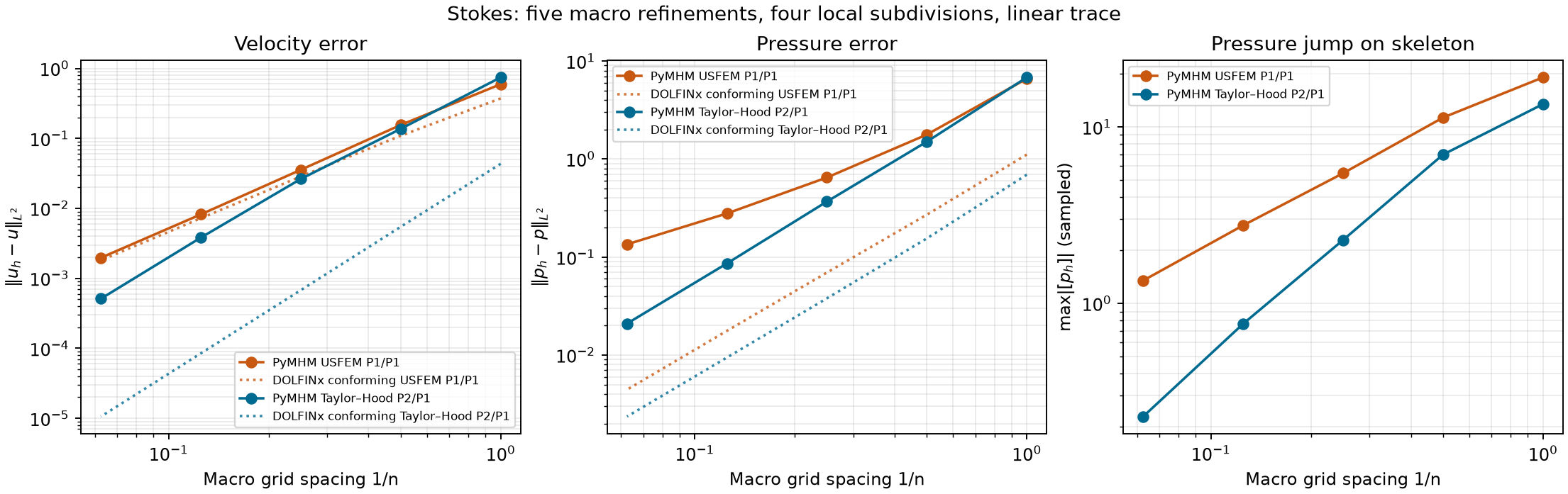
The dotted conforming references use the same microtriangles but different continuity and boundary constraints. For example, at \(n=4\), their pressure errors are 0.0695747 (P1/P1) and 0.0379456 (P2/P1), compared with 0.648499 and 0.368393 for the corresponding MHM configurations. The comparison exposes the cost of the selected skeleton/local approximation; it is not an equality test.

Local refinement alone is insufficient

With \(n=4\) and the linear skeleton fixed, increasing the local subdivisions through 4, 6, 8, 12, and 16 reduces the USFEM pressure error from 0.648499 to 0.373590. Taylor–Hood changes from 0.368393 to 0.366639. The latter is already limited primarily by the trace approximation on this sequence.

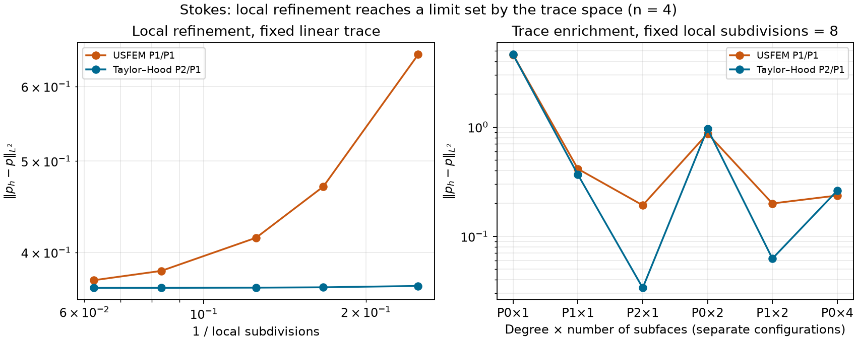
At eight local subdivisions, replacing the single linear trace by a quadratic trace reduces the pressure error from 0.414425 to 0.192241 for USFEM, and from 0.366859 to 0.0336089 for Taylor–Hood. Splitting each face into two subfaces with linear traces gives 0.199718 and 0.0623463. These are separate configurations, not equally spaced samples of one refinement parameter.

Enrichment must remain compatible with the local spaces. The solver requires a full-rank gauged system. For example, P1/P1 locals with only two subdivisions and a linear trace are insufficient in the \(n=4\) configuration. Even on the two-macrotriangle mesh, its local trace coupling has rank 10 for 12 trace columns; the gauged global matrix has rank 23 out of 25. With four local subdivisions those ranks become 12 and 25. Independent singular-value checks confirm this loss of trace control, including at zero drag; switching the linear-solver backend cannot restore the missing rank.

Pressure profiles retain the discontinuities

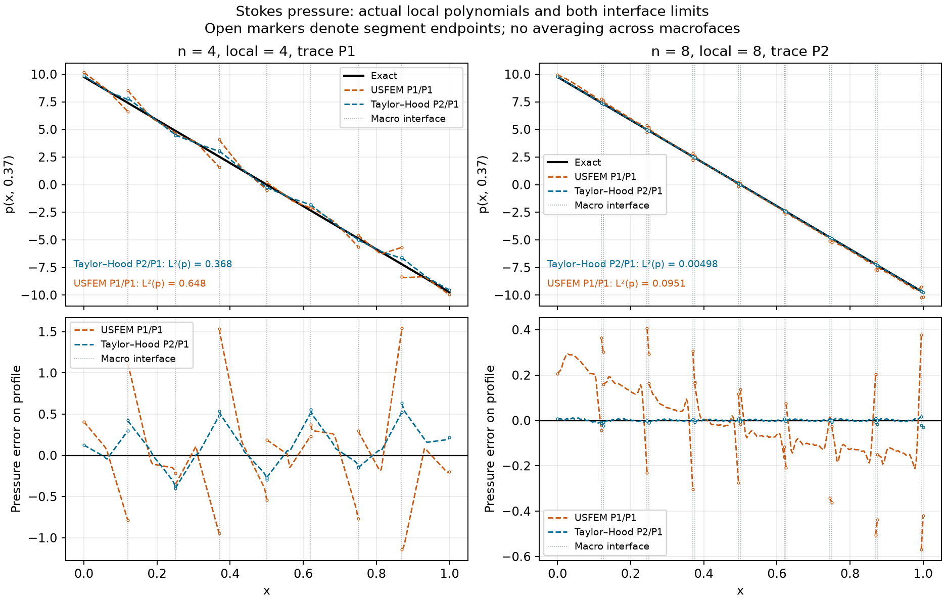
Local pressure is continuous inside each macrocell, but is not constrained to be continuous across macrofaces. The plot below evaluates both one-sided limits at each crossing of \(y=0.37\). Each curve ends at its macrocell boundary; no averaging joins the pressure traces. Open markers make those boundaries visible. The lower panels have different vertical ranges to retain the refined error.

Configuration	Method	Pressure \(L^2\) error	Relative pressure error	Maximum sampled skeleton jump
\(n=4\), local 4, trace P1	USFEM P1/P1	0.648499	5.188%	5.46376
\(n=4\), local 4, trace P1	Taylor–Hood P2/P1	0.368393	2.947%	2.28791
\(n=8\), local 8, trace P2	USFEM P1/P1	0.0951284	0.761%	1.20411
\(n=8\), local 8, trace P2	Taylor–Hood P2/P1	0.00497627	0.0398%	0.0776261

The jump statistic samples every internal macroface; it is not confined to the profile, and it is not a certified supremum. The squared jump integral is also recorded, integrating separately over each microedge. The refined USFEM pressure has visible localized errors, despite its smooth velocity field. Pressure accuracy is measured by its own errors and jump norms.

The 2017 published refinement experiments use equal-order local polynomials of degree \(\ell+2\) on a single local element for skeleton degree \(\ell\). The native P1/P1 experiment above does not match those spaces, and is not a reproduction of its published convergence curves. Remark 4 discusses equal local and trace degree on sufficiently refined local meshes as a numerical observation requiring further theoretical investigation. A successful rank check does not provide that missing uniform stability result. The higher-order paper comparison uses those local spaces through pyMHM's DOLFINx/UFL adapter and compares with digitized article data. It matches the published P2/P2 velocity, pressure and standard H(div) stress curves at six levels within the figure's digitization precision. P3/P3 velocity and pressure also agree at six published levels. Discrepancies in the full stress L2 norm and the P3/P3 stress H(div) norm remain explicit in that comparison.

Numerical records and figures

Measurements and separate profile segments are available in examples/results/flow-audit.json. Render its figures without repeating finite element solves:

pixi run --locked -e notebooks python -m examples.plot_flow_audit

The uncondensed check and global reference used SciPy's sparse direct solver independently of the package's linear-solver adapter.

References

• Rodolfo Araya, Christopher Harder, Abner H. Poza, and Frédéric Valentin (2017). Multiscale hybrid-mixed method for the Stokes and Brinkman equations—The method, Computer Methods in Applied Mechanics and Engineering 324, 29–53. DOI: 10.1016/j.cma.2017.05.027.