Stabilized Oseen flow and two-level adaptivity

The Oseen implementation solves

\[ -\nu\Delta u+(\beta\cdot\nabla)u+\gamma u+\nabla p=f, \qquad \nabla\cdot u=0, \]

with the velocity-gradient viscous operator. Local continuous equal-order \(P_k/P_k\) spaces, independent vector-valued skeletal spaces, and the stabilization of Araya, Cárcamo, Poza and Valentin (2021) are available through solve_brinkman(..., formulation="oseen", degree=k). The global hybrid problem retains translation moments, including for positive reaction; reconstructed pressure uses the prescribed global mean when all velocity components have Dirichlet data.

Variable convection and local stabilization

A constant convection vector needs no derivative data. For a callable advection(points), supply its analytical divergence through advection_divergence and a finite global bound on its Euclidean magnitude through advection_bound. The latter is required by the stabilized Oseen formulation. The Taylor–Hood formulation accepts variable convection without this stabilization bound. Bounds are checked at integration points; sampling cannot prove a bound everywhere.

The skew convection form uses the reaction correction \(\gamma-\tfrac12\nabla\cdot\beta\), so its strong operator remains \((\beta\cdot\nabla)u+\gamma u\). The local residuals are

\[ R(u,p)=-\nu\Delta u+\nabla u\,\beta+\gamma u+\nabla p, \qquad R^*(v,q)=-\nu\Delta v-\nabla v\,\beta+\gamma v+\nabla q. \]

With the pressure-test sign convention used by the package, the stabilized terms are \(\kappa_\tau(\nabla\cdot u,\nabla\cdot v)_\tau -\delta_\tau(R(u,p),R^*(v,q))_\tau\), and the source contribution includes \(-\delta_\tau(f,R^*(v,q))_\tau\). These signs and both convection directions are checked against independently assembled DOLFINx/UFL operators for degrees one, two and three, including variable convection.

Let \(h_\tau\) be the fine-cell diameter, \(m_\tau=\min(1/3,C_\tau)\), where \(C_\tau h_\tau^2\|\Delta v\|^2\leq\|\nabla v\|^2\). Writing \(d=4\nu/m_\tau\) and \(b=h_\tau\|\beta\|_{\infty,\tau}\), equations (26)–(27) give

\[ \delta_\tau=\frac{h_\tau^2} {\max(\gamma h_\tau^2,d)+\max(d,b)}, \qquad \kappa_\tau=b\min(1,b/d). \]

The implementation accepts constant nonnegative scalar \(\gamma\) for this formulation. Its analytical reliability assumptions are stronger: \(\gamma-\tfrac12\nabla\cdot\beta\geq\gamma_m>0\). The internal-layer example has \(\gamma=0\), as in the article, and is outside that strict coercivity hypothesis. A computed estimator or small linear-system residual does not establish the theorem's assumptions.

Residual estimator and adaptive spaces

estimate_flow_error evaluates the two levels of the Oseen estimator in (33)–(34), or the Stokes–Brinkman estimator when variant="stokes-brinkman-2021". These interfaces currently require full Dirichlet boundaries, constant positive viscosity and uniform skeletal degree \(\ell\). Local meshes may have different refinements. Face quadrature is partitioned at the local-cell and skeletal breakpoints, preserving one-sided velocity values.

The first level uses \(-[u_h]/2\) on internal macrofaces and \(g-u_h\) on the exterior. Its denominator is the original macroface length, including when the trace is subdivided. An interior macroface appears twice in the sum of macrocell boundaries. The second level contains momentum residuals, divergence, and pseudotraction mismatches on local faces. The residual uses the sign-reversed pseudotraction \(\nu\nabla u\,n-pn-u(\beta\cdot n)/2\). For Oseen,

\[ \eta_2=2^{-2\ell}\Big(\sum_K\eta_{2,K}^2\Big)^{1/2}, \qquad \eta=\eta_1+\eta_2. \]

The Stokes–Brinkman variant has no \(2^{-2\ell}\) factor. These are estimators with constants and higher-order terms in their respective bounds; the reported value is not a certified upper bound with constant one. Discontinuous material coefficients must align with the local cells for the Gaussian volume quadrature used by this estimator.

adapt_flow uses equation (52): \(\eta_F=(\sum_{\widetilde F}\eta_{1,\widetilde F}^2)^{1/2} +\sum_{K\in\omega_F}\eta_{2,K}\), with unscaled local indicators. It marks macrofaces above a fraction of the maximum indicator and bisects segments with maximal contribution on those faces. Local meshes double when the second level dominates; an explicit uniform-grid closure also resolves every new trace breakpoint. Thus the macro topology stays fixed while local meshes and traces adapt. max_local_refinement imposes a declared resolution limit and returns a distinct stop reason.

The example helpers below are repository sources, supplied separately from the installed library. Open the corresponding notebook to acquire its verified companion, as described in the notebook guide.

import numpy as np
from pymhm import TriangleMesh
from pymhm.adaptivity.flow import adapt_flow
from examples.formulations.application import flow as solve_equations

result = adapt_flow(
    TriangleMesh.unit_square(2),
    solve_step=solve_equations,
    formulation="oseen",
    degree=3,
    drag=2.0,
    advection=lambda x: x,
    advection_divergence=2.0,
    advection_bound=np.sqrt(2.0),
    source=lambda x: 2.0 * x,
    iterations=3,
    theta=0.5,
)

solve_step builds the current mathematical velocity/pressure equations through the public provider; the shared adaptive owner supplies refinement and estimator checks. The callback receives the actual oriented trace and local partitions. The same contract applies to macro refinement through adapt_flow_macros.

Analytical campaigns

examples/solve_oseen.py runs the original package implementation on the smooth, boundary-layer and internal-layer data from sections 5.1–5.3. The smooth study uses \(P_3/P_3\) local spaces with one fine triangle per macrocell, crisscross meshes with \(H=1/2,1/4,1/8,1/16,1/32\), and pressure \(p=(x-y)^6-1/28\). Viscosity and trace-degree studies are separate campaigns. The variable-convection experiment is supplementary: \(\beta=(x,y)\) and \(\gamma=2\), with the source differentiated from the same exact fields.

The boundary-layer experiment uses \(\nu=0.01\), \(\gamma=1\), \(\beta=(1,1)/\sqrt2\), and \(p=(x-y)^8-1/45\). The internal-layer experiment uses \(\nu=0.001\), \(\gamma=0\), \(\beta=(1,0)\), and the published hyperbolic-tangent streamfunction. Both adaptive studies keep 16 initial macrotriangles, use \(P_3/P_3\) locally and \(P_1\) skeletal segments, and state their marking threshold and quadrature in each record.

The experiments reproduce the stated analytical problems and stabilized forms. Historical adaptive connectivity and marking parameters are not fully specified by the article; the archived campaigns do not assert an identical adaptive mesh or reproduction of its numerical tables. Physical errors are integrated on local cells, separately from the polynomial samples used for spatial plots. The mixed norm is

\[ \|(e_u,e_p)\|_{V\times Q}^2= \operatorname{diam}(\Omega)^{-2}\|e_u\|_{L^2}^2+ \|\nabla e_u\|_{L^2}^2+\|e_p\|_{L^2}^2. \]

Run an acquisition with the test environment, and render its archived data with the notebook environment. Large convergence studies are separate from routine CI; CI covers analytical patches, exact estimator moments, marking, and small adaptive solves.

pixi run --locked -e test-core python -m examples.solve_oseen --case smooth --levels 2 4 8 16 32
pixi run --locked -e test-core python -m examples.solve_oseen --case boundary --viscosity .01 --levels 2 --adaptive --iterations 4 --order 20
pixi run --locked -e notebooks python -m examples.plot_oseen

Archived results

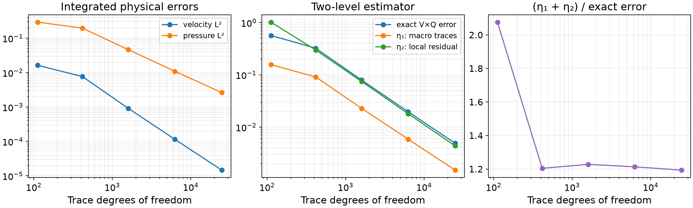
All eight studies contain five solved states. The uniform studies below use \(H=1/32\) at their last state; the adaptive studies retain their original 16 macrotriangles. Errors are absolute physical \(L^2\) norms.

Study	Viscosity	Trace degree	Final velocity error	Final pressure error	Final effectivity
Smooth	1	0	2.46134e-3	1.58417e-1	0.9406
Smooth	1	1	1.47070e-5	2.62523e-3	1.1940
Smooth	1	2	2.24595e-7	1.05024e-4	1.1340
Smooth	0.01	1	1.26142e-4	2.00064e-4	0.3479
Smooth	0.0001	1	2.20335e-3	6.26125e-4	0.2689
Variable convection	1	1	1.48474e-5	2.63794e-3	1.1854
Adaptive boundary layer	0.01	1	9.00694e-3	8.15895e-3	0.1592
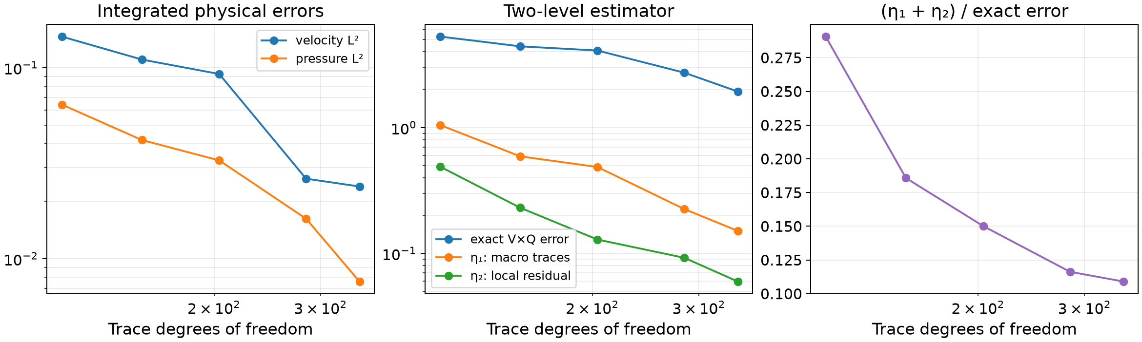
Adaptive internal layer	0.001	1	2.38814e-2	7.59098e-3	0.1090

The effectivity variation matters: these data do not establish a universal viscosity-independent estimator constant. The boundary and internal-layer runs reduce their errors but retain finite discretization error. Their final local meshes contain 2,566 and 2,917 triangles, respectively. Their recorded algebraic residuals are below \(6\times10^{-15}\); this is a separate check from their approximation errors.

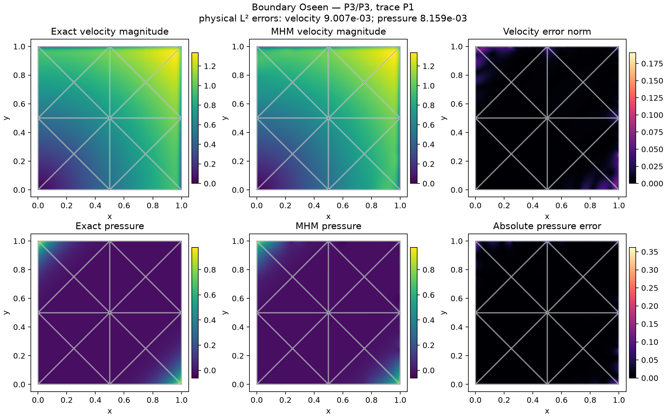
The spatial-map record identifies the P3/P3 boundary-layer case at viscosity \(0.01\), its P1 trace and four adaptive iterations. Its 2,566 fine triangles and physical norms agree with the retained configuration; the largest norm difference is below \(3\times10^{-13}\) relatively.

References

• Rodolfo Araya, Cristian Cárcamo, Abner H. Poza, and Frédéric Valentin (2021). An adaptive multiscale hybrid-mixed method for the Oseen equations, Advances in Computational Mathematics 47, article 15. DOI: 10.1007/s10444-020-09833-8.