Adaptive Darcy macro meshes

solve_adaptive_darcy combines the material-weighted energy estimator, bulk marking and conforming triangular macro refinement. This is an original adaptive policy using the reconstruction and estimator of Barrenechea et al. (2026). The example uses their smooth problem in §6.1; its adaptive meshes and marking sequence are specified here rather than attributed to a published figure.

On the unit square,

\[ p=\sin(2\pi x)\sin(2\pi y),\qquad K=I,\qquad f=8\pi^2p,\qquad p|_{\partial\Omega}=0. \]

Estimator and refinement policy

Let \(s_h\) be the conforming Oswald potential and \(q_h^R\) the RT moment reconstruction. The macro indicators use the weighted flux defect, nonconformity, reconstructed-divergence defect and data oscillation:

\[ \begin{aligned} \eta_K^2&=(\eta_{1,K}+\eta_{3,K}+\mathrm{osc}_K)^2+\eta_{2,K}^2,\\ \eta_{1,K}&=\|K^{-1/2}(K\nabla p_h+q_h^R)\|_K,\\ \eta_{2,K}&=\|K^{1/2}\nabla(p_h-s_h)\|_K. \end{aligned} \]

The remaining two terms carry the convex-cell Poincaré factor \(\operatorname{diam}(K)/(\pi\sqrt{\alpha_K})\), where \(\alpha_K\) is a certified lower material eigenvalue. The underlying estimator and reconstruction retain their boundary-representability, continuous-test equilibrium and integration requirements. Numerical quadrature is not interval arithmetic.

Both adaptive entry points accept estimator_convention="published" to use the literal equations (5.3)–(5.7), with an unweighted L2 flux defect and diameter/π in the divergence and oscillation terms. The default "energy" uses the material weights above. The conventions coincide for this unit-diffusion example; their heterogeneous meanings and coefficient scalings are documented separately. Changing that option changes marking values, not the finite-element PDE.

mark_dorfler selects the smallest number of cells whose squared indicators sum to at least \(\theta\sum_K\eta_K^2\). Ties retain cell order. Selected triangles undergo red refinement into four children. Closure promotes any neighbor with two bisected edges to red refinement; single-edge neighbors use two green children. Shared midpoint indices guarantee conformity. Existing skeletal partitions follow their physical parent faces, while new interior faces receive the requested degree and segmentation. Neumann classifications and local ellipticity bounds follow the same ancestry.

This policy does not imply an error-contraction or optimal-complexity theorem. Repeated green refinement does not provide a mesh-independent minimum-angle guarantee. The campaign records the shape quality \(4\sqrt3 |K|/\sum_{F\subset\partial K}|F|^2\), alongside the numerical error.

The alternative macro_refiner=refine_longest_edge follows longest-edge propagation paths. It bisects a boundary edge or an edge longest in both incident triangles, then repeats until every marked triangle has been replaced. Every intermediate partition is conforming. The algorithm's exact-arithmetic angle bound is half the initial minimum angle (Rivara (1984)); floating-point coordinates remain subject to the mesh validity checks. Cell and face ancestry is preserved through the entire propagation path. This geometric bound is separate from any claim about estimator contraction.

The example helpers below are repository sources, supplied separately from the installed library. Open the corresponding notebook to acquire its verified companion, as described in the notebook guide.

import numpy as np
from pymhm import TriangleMesh
from pymhm.adaptivity.darcy import solve_adaptive_darcy
from examples.formulations.application import darcy as solve_equations

result = solve_adaptive_darcy(
    TriangleMesh.unit_square(2), solve_step=solve_equations,
    iterations=5, theta=0.5,
    trace_degree=1, degree=3, reconstruction_degree=2,
    local_refinement=2, quadrature_order=10, estimator_order=10,
    source=lambda x: 8*np.pi**2*np.prod(np.sin(2*np.pi*x), axis=1),
)
print(result.totals)

solve_step receives the current mesh, oriented skeleton, physical data and local partitions. The editable application.darcy helper composes the public mathematical provider with generic assembly, pressure constraints and field recovery. Users may supply their own callback with the same contract. The shared adaptive owner retains marking, boundary ancestry and estimator checks.

A local_mesh_factory(macro_mesh, cell_index) may construct fresh material-fitted local meshes at each level. A fixed list of local meshes cannot survive changing macro geometry and is rejected by the adaptive wrapper. All fine meshes must form a globally conforming partition for potential recovery. The current driver refines macro geometry while keeping local degree and nominal local refinement fixed.

Balancing local and macro refinement

solve_balanced_adaptive_darcy additionally compares \(\|\eta_3+\mathrm{osc}\|_{\ell^2}\) with a declared multiple of \(\sqrt{\|\eta_1\|_{\ell^2}^2+\|\eta_2\|_{\ell^2}^2}\). When the former is larger, it doubles the local refinement uniformly; otherwise it marks macroelements. Uniform local refinement preserves shared fine-edge partitions. A three-argument factory factory(mesh, cell, refinement) can supply a nested material-fitted local hierarchy. Returned local_refinements, decisions and stop_reason state which operation was performed and whether a local or macro budget terminated the loop.

These terms are refinement proxies, not an exact decomposition into local and global discretization errors. In particular, the divergence term contains a macro-diameter Poincaré bound and need not decrease under local refinement for rough coefficients. The policy does not establish estimator contraction or replace comparison with an independently refined reference. It stops explicitly when the allowed local resolution is exhausted.

An optional local_error_indicator(solution) supplies a separate local-resolution measurement. estimate_darcy_local_refinement uniformly red-refines each local mesh, solves the same Neumann problem with the current skeletal flux, and measures the material-weighted gradient difference through exact parent-child ancestry. The source, material, pressure degree and trace data stay fixed. Pressure means do not affect this seminorm. The returned local_squared values and total measure an actual difference between two local approximations; interpreting it as a local-error bound would additionally require a saturation estimate. The SPE10 adaptive case uses this option with material-fitted local meshes, rather than identifying the divergence term with local error.

Five-level numerical campaign

Both sequences start with eight macrotriangles and use \(\theta=0.5\), local refinement 2, \(k=\ell+2\), and RT2 reconstruction. Assembly and estimator integration use order 10; the energy error is independently integrated at orders 12 and 14. Global counts include skeletal coefficients and one retained pressure mean per macrocell.

Trace degree	Level	Macro cells	Global unknowns	Energy error	Estimator
0	0	8	24	1.83747	5.59985
0	1	24	66	2.03506	4.73439
0	2	42	111	1.83059	3.43188
0	3	76	200	1.64864	3.62696
0	4	138	358	1.34303	2.81170
1	0	8	40	1.80008	2.39124
1	1	24	108	0.881408	1.49612
1	2	44	192	0.353029	1.43926
1	3	60	256	0.258595	0.553251
1	4	116	486	0.175916	0.394598

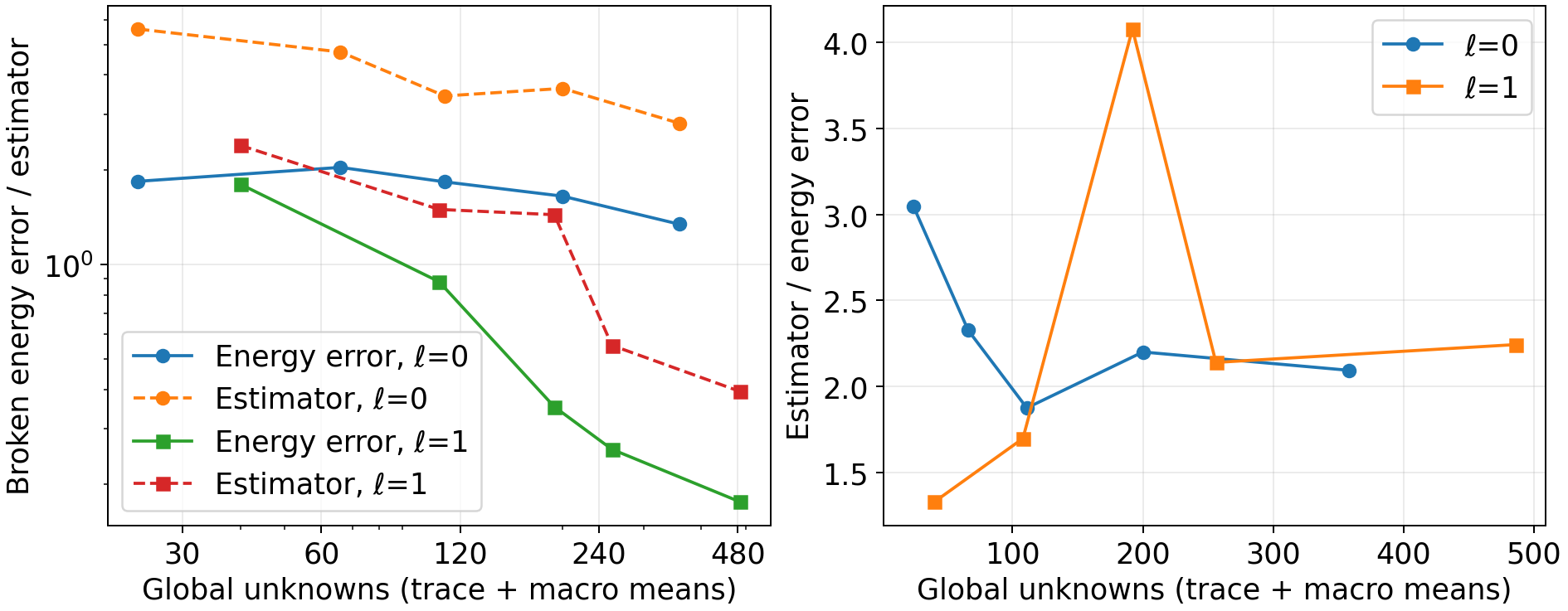
The P0 trace sequence is not monotone: its first refinement raises the energy error, and a later refinement raises the estimator. This reflects the recorded sequence of different hybrid spaces; these spaces are not asserted to be nested. The P1 trace sequence reduces the measured energy error by a factor of about 10.2 over five solves. These observations are not universal convergence rates.

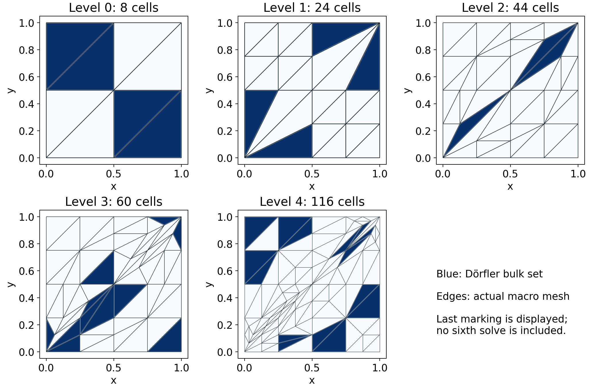
The last panel also displays the next marking set, but no sixth solve is included. The lowest recorded shape quality in this sequence is 0.1271. Geometry closure can refine cells outside the selected bulk set.

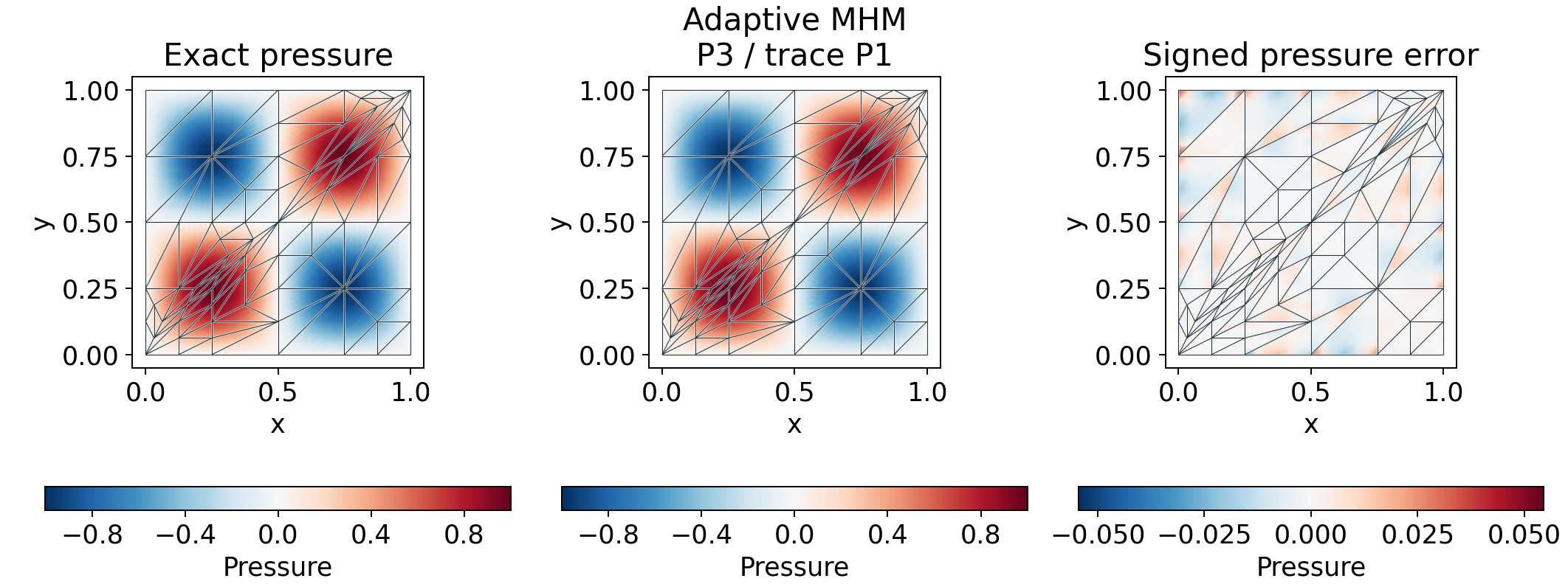
The exact and numerical pressures share a color scale. The error has its own symmetric scale, and all panels retain the actual macro boundaries. Broken fine-element values remain independent at interfaces.

Reproduction and scope

pixi run --locked -e notebooks python -m examples.adaptive_darcy_campaign --collect
pixi run --locked -e notebooks python -m examples.adaptive_darcy_campaign

Records and sampled fields are in examples/results/adaptive-darcy. Notebook 39 presents the smooth adaptive example; Notebook 38 treats material-fitted local approximation. Light CI checks cover conformity, ancestry, deterministic bulk marking, mixed boundary transfer and the measured estimator bound on small analytical cases. The five-level campaign is executed separately. No SPE10 adaptive result is inferred from this smooth example.

References

• Gabriel R. Barrenechea, Larissa Martins, Weslley Pereira, and Frédéric Valentin (2026). An H(div; Ω)-Conforming Flux Reconstruction for the Multiscale Hybrid-Mixed Method, Multiscale Modeling & Simulation 24(2), 399–428. DOI: 10.1137/24M1673073.

• M. Cecilia Rivara (1984). Algorithms for refining triangular grids suitable for adaptive and multigrid techniques. International Journal for Numerical Methods in Engineering 20(4), 745–756. DOI: 10.1002/nme.1620200412.