RT flux reconstruction by moments

reconstruct_darcy_moments implements the face and volume moments in Barrenechea et al. (2026), equations (4.9) and (5.1). It takes a primal MHM pressure and constructs a globally H(div)-conforming Raviart–Thomas flux. Mathematical orders RT0, RT1 and RT2 are available on affine triangles. The RT2 vector space has 15 degrees of freedom per triangle: three normal moments on each edge and six interior vector moments.

This is separate from the energy-based RT0 reconstruction. The moment construction does not solve an equilibrium minimization problem and does not impose an independent mass balance in every fine cell.

Definition and signs

Let \(q_h=-K\nabla p_h\) be the broken primal flux. On a fine triangle \(T\), construct \(\sigma_h\in\mathrm{RT}_m(T)\) from

\[ \begin{aligned} \int_e\sigma_h\cdot n_e\,\mu &=\int_e\lambda_h^{(n_e)}\,\mu, &&e\subset\partial K,\\ \int_e\sigma_h\cdot n_e\,\mu &=\int_e\{q_h\}\cdot n_e\,\mu, &&e\subset\operatorname{int}K,\\ \int_T\sigma_h\cdot v &=\int_Tq_h\cdot v, &&v\in[\mathbb P_{m-1}(T)]^2. \end{aligned} \]

The face test functions satisfy \(\mu\in\mathbb P_m(e)\), and braces denote the arithmetic average of the two physical one-sided values. The notation \(\lambda_h^{(n_e)}\) means the skeletal normal flux expressed in the direction \(n_e\). pyMHM stores \(\lambda_h=q\cdot n_e\) relative to the global face normal. The paper uses the opposite multiplier sign, hence its boundary formula contains \(-\lambda_H\). Oriented normal moments and the contravariant Piola transform account for local outward normals and polynomial reversal.

The skeletal degree must not exceed \(m\), and every skeletal partition point must coincide with a fine boundary vertex. The native wrapper requires \(m\leq k\), where \(k\) is the primal pressure degree. The optimal flux estimates in the paper additionally assume \(k\geq\ell+2\) in two dimensions, where \(\ell\) is the skeletal degree, together with the stated mesh, coefficient and solution regularity assumptions. In particular, Theorem 4.7 assumes diffusion polynomial on each fine triangle, \(p\in H^{k+1}(K)\) and \(K\nabla p\in H^{\ell+1}(K)^2\cap H(\operatorname{div};K)\). An accepted API input alone does not establish those estimates.

The example helpers below are repository sources, supplied separately from the installed library. Open the corresponding notebook to acquire its verified companion, as described in the notebook guide.

import numpy as np
from pymhm import FaceSpace, SkeletonSpace, TriangleMesh
from examples.formulations.application import darcy as solve_darcy
from pymhm.recovery.moments import reconstruct_darcy_moments

mesh = TriangleMesh.unit_square(4)
skeleton = SkeletonSpace(mesh, tuple(FaceSpace.uniform(1) for _ in mesh.faces))
pressure = solve_darcy(
    mesh, skeleton=skeleton, degree=3, local_refinement=2,
    source=lambda x: 8*np.pi**2*np.sin(2*np.pi*x[:, 0])*np.sin(2*np.pi*x[:, 1]),
    quadrature_order=8,
)
flux = reconstruct_darcy_moments(pressure, degree=2)

For a custom local discretization, reconstruct_flux_moments accepts one raw_flux(points, fine_cell_indices) evaluator per macrocell. This allows explicit one-sided values for a discontinuous material. The native wrapper can use the same evaluators through raw_fluxes. Its default permeability callback is evaluated at the actual physical face points; when permeability jumps across an interior fine face, supply the one-sided evaluators. No coordinate perturbation or averaging of material coefficients is inferred. Discontinuities solely on macrofaces are handled by the skeletal normal data.

What is conserved

Proposition 4.3 concerns the continuous macro-local test space:

\[ (\operatorname{div}\sigma_h-f,v)_K=0, \qquad v\in C^0(K)\cap\mathbb P_m(\mathcal T_h^K). \]

For \(m=0\), that space contains one constant per macrocell. It does not contain independent constants on each fine triangle. Accordingly:

Method	Quantity
`continuous_moment_residuals()`	Moments against continuous local Pm
`conservation_residuals()`	Integrated balance per macrocell
`fine_conservation_residuals()`	Measured fine-cell balance defects, generally nonzero
`normal_flux_residuals()`	Boundary normal moments minus the skeletal moments
`divergence_l2_error(f)`	Error of the raw RT divergence
`projected_divergence_l2_error(f)`	Error of its L2 projection onto continuous local Pm

The continuous projection satisfies the higher-order approximation property in Theorem 4.4. It is not the raw RT divergence. When a macrocell contains only one fine triangle, the two polynomial spaces coincide and the distinction disappears. Diagnostics use the recorded reconstruction quadrature; a higher order error norm measures approximation independently. Nonpolynomial inputs retain the usual quadrature error.

Smooth sine study

Use the analytical data of section 6.1,

\[ p=\sin(2\pi x)\sin(2\pi y),\qquad K=I,\qquad f=8\pi^2p, \]

with zero boundary pressure. The study compares \((\ell,k)=(0,2)\) and \((1,3)\), RT2 reconstruction, and four fine triangles per macrotriangle. There are five macro grid resolutions, \(n=1,2,4,8,16\), with the diagonal triangulation defined by TriangleMesh.unit_square. Assembly uses quadrature order eight and physical error norms use order ten.

These are pyMHM analytical results. They do not claim agreement with digitized ordinates or execute the paper's FreeFem++ implementation.

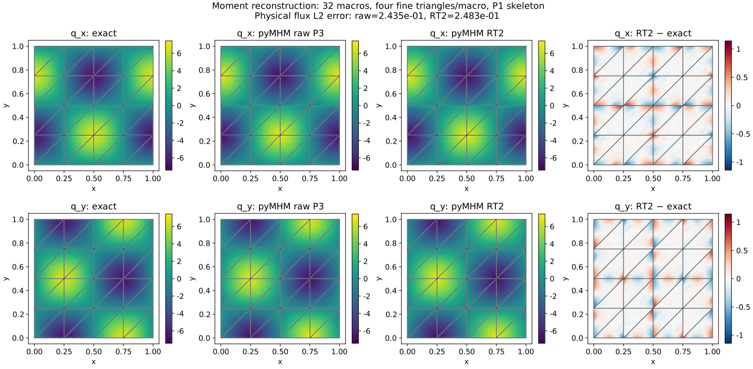
Physical flux, broken primal field and moment-reconstructed RT2 field

The flux map uses 32 macrotriangles, P1 skeletal traces and P3 primal locals. It preserves separate fine-cell values. Every analytical, numerical and error panel displays the actual macro mesh; exact and numerical flux panels share color scales. The reconstruction enforces normal conformity but does not promise a smaller L2 error for every finite discretization.

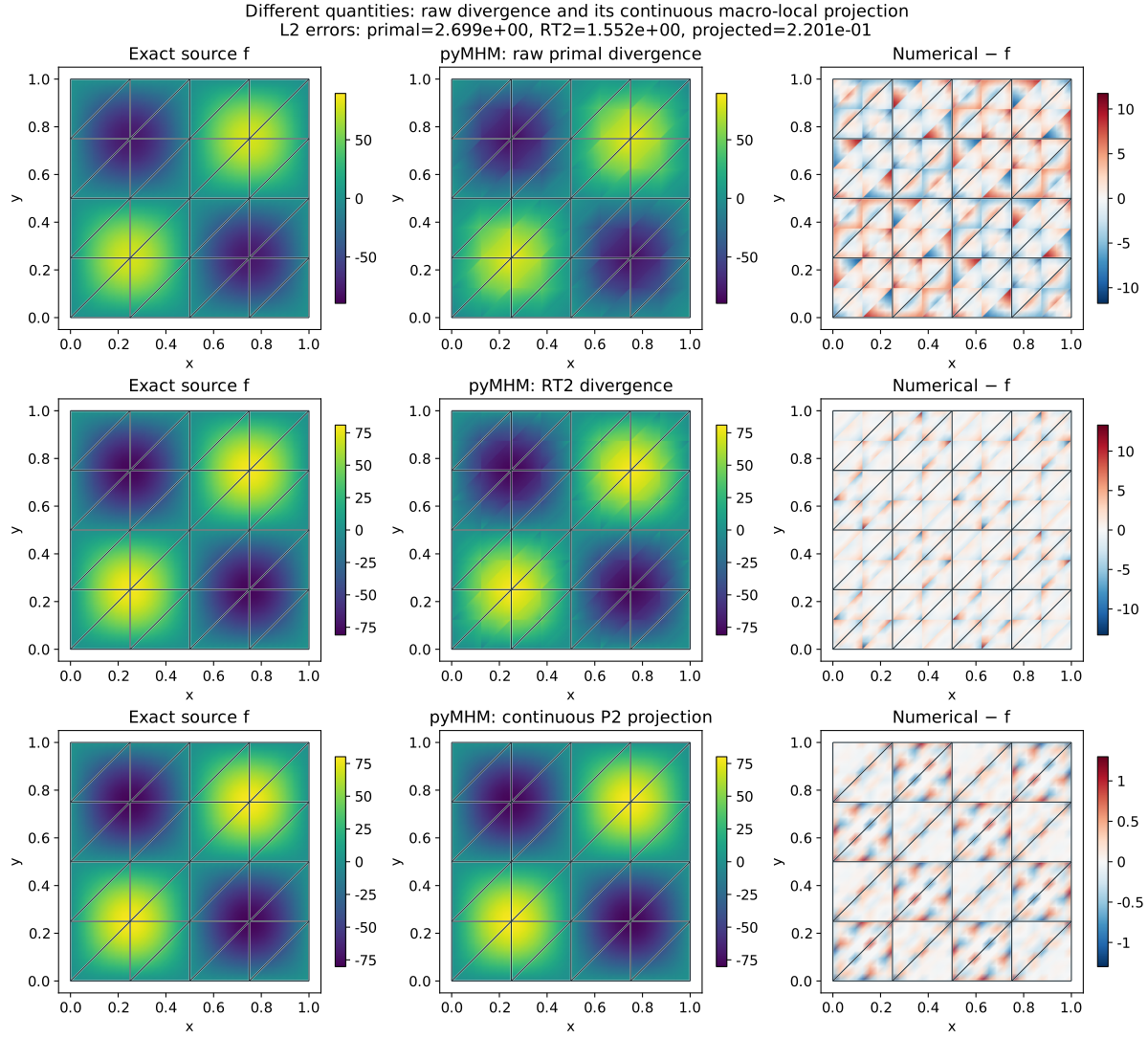
Raw primal divergence, raw RT divergence and its continuous projection

The last row is a projection, explicitly identified as such. At this mesh, the L2 divergence errors are 2.69947 for the primal flux, 1.55194 for the RT2 flux, and 0.220082 for the continuous P2 projection. The flux L2 errors are 0.243490 and 0.248253 respectively: normal conformity and divergence accuracy improve here without a flux L2 improvement.

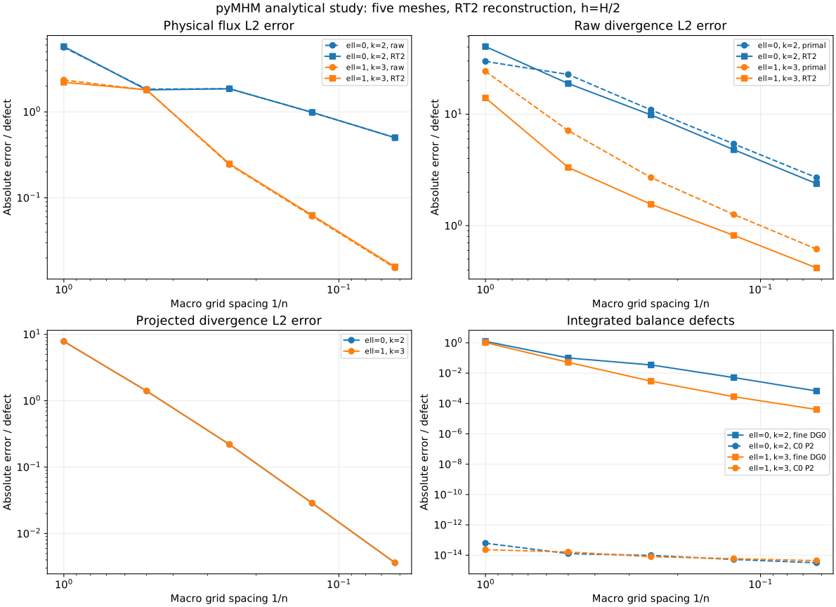
Five-level flux and divergence convergence with separate balance diagnostics

At the finest level the measured errors are:

Skeletal / primal degrees	Raw flux L2	RT2 flux L2	Raw RT2 divergence L2	Projected divergence L2
P0 / P2	0.501010	0.500989	2.37786	0.00362392
P1 / P3	0.0152811	0.0157188	0.416997	0.00362392

The projected-divergence rate between the final two meshes is 2.984. All continuous moments in the study are below \(6.2\times10^{-14}\), while the fine-cell integrated defects at the finest level are \(6.63\times10^{-4}\) and \(4.01\times10^{-5}\), respectively.

The two projected-divergence curves overlap because both satisfy the same continuous P2 moments of the same source on the same mesh. Coarse under-resolved levels can have nonmonotone flux or pressure errors. The fine-cell integrated defects shown in the last panel are generally nonzero, consistently with equilibrium against continuous macro-local tests. Spatial maps sample each fine triangle on sixteen display triangles, without merging one-sided traces; quadrature norms are independent of that display interpolation.

Verification and scope

Portable tests check canonical RT duality, Piola orientation, polynomial reproduction, divergence-commuting interpolation, all volume moments, normal continuity within and between macrocells, continuous-test equilibrium, and nonzero fine-cell defects. Three native DOLFINx/Basix RT tests independently compare physical interpolation and UFL divergence for RT0, RT1 and RT2. Basix numbers those spaces with degrees 1, 2 and 3 respectively. The divergence is compared through its exact discontinuous polynomial representation, without smoothing.

The implemented orders and affine triangular geometry are explicit limits. The moment flux alone is not a complete guaranteed a posteriori estimator: the paper also requires a conforming potential reconstruction, divergence correction and data oscillation terms with their assumptions.

pixi run --locked -e notebooks python -m examples.plot_reconstruction_moments

The archived numerical records and notebook 18_reconstruction_moments.ipynb expose the measured errors and conservation quantities.

References

Gabriel R. Barrenechea, Larissa Martins, Weslley Pereira, and Frédéric Valentin (2026). An H(div; Ω)-Conforming Flux Reconstruction for the Multiscale Hybrid-Mixed Method, Multiscale Modeling & Simulation 24(2), 399–428. DOI: 10.1137/24M1673073.