Material interfaces inside macroelements
The two-layer problem in §6.2 of Chaumont-Frelet, Paredes and Valentin (2026) isolates the role of the skeletal partition. On the unit square,
Pressure and normal physical flux are continuous across the material interface; the normal pressure derivative generally jumps. Coordinates and coefficients are dimensionless.
This case has been executed and checked against an analytical reference and selected published numerical values. It is not a complete reproduction of the article. The S0 and S1 gradient errors agree closely with the rounded values in Figure 5; the S2 curve agrees in its lower sensitivity to the perturbation, but not in all its numerical values. The comparisons below distinguish these two statements. The 2022 preprint Chaumont-Frelet, Paredes and Valentin (2022, preprint v1) is an earlier version of the same work; the numerical target is the final 2026 publication Chaumont-Frelet, Paredes and Valentin (2026), §6.2 and Figures 4–6, printed pages 24–26.
The macro mesh contains 16 crisscross triangles. S0 uses a middle row at \(y=1/2\). S1 moves that row to \(1/2+\delta\), retaining one polynomial multiplier per original macroface. S2 uses the same perturbed geometry and splits each multiplier face where it crosses the physical interface. The macro triangles remain unchanged between S1 and S2. This is the distinction in the article's Figures 4–6.
| Feature | Published target | This numerical study |
|---|---|---|
| PDE, boundary data and contrast | Unit square, source 1, zero pressure, lower/upper coefficients 10/1 | Same data |
| Macro partition | 16 crisscross triangles; perturb the middle row | Explicit 16-triangle construction; the four square centers move with their rows |
| Skeleton | Degree 2; S2 splits material crossings | Discontinuous degree-2 polynomials on each segment; seven new breakpoints in S2 |
| Local solves | Sufficiently accurate; local degree and mesh not specified numerically | Continuous P4 on individually material-fitted meshes, with initial refinement 4, 8 or 16 |
| Reference for errors | Standard continuous piecewise-linear Galerkin reference on 1,048,576 material-fitted squares | Independently derived Fourier solution, with truncation and quadrature checks; separate Q1 refinement sequence |
Here “unfitted” refers primarily to the macro partition. The displayed main campaign deliberately fits the local approximation meshes to the material interface. An additional campaign keeps local triangles unfitted and integrates their material intersections exactly; its error is shown separately below.
The theoretical mechanism is that each skeletal subface belongs to one physical material region. Theorem 2 and equation (20) of Chaumont-Frelet, Paredes and Valentin (2026) use piecewise regularity on the physical partition, positive coefficient bounds and geometric regularity. For \(0\le q\le\ell\), the estimate assumes \(p\in H^{q+3}(\mathcal P_\Omega)\), \(a\in W^{q+1,\infty}(\mathcal P_\Omega)\) and \(a\nabla p\in H(\mathrm{div},\Omega)\). Its constants include the physical-region extension bounds, macrocell shape regularity and macro-mesh quasi-uniformity (§§3.1–3.2). In three dimensions the skeletal projection constants also depend on subface geometry (Remark 1); arbitrary thin cut polygons do not have a uniform constant merely because they fit the material. The results do not cover a multiplier segment that straddles an unresolved coefficient jump. S1 is such a diagnostic configuration; S2 restores the fitted-subface condition. The theorem analyzes exact local problems. The finite P4 local solves add a discretization error, which must be examined independently. Neither the theorem nor this one-contrast experiment proves contrast-independent accuracy for arbitrary cuts or materials.
Integration, local approximation and skeletal approximation
These are three independent operations:
material_triangle_quadratureintegrates each fine triangle on its intersections withCartesianCellFieldpixels. The scalar primal, RT0, BDM2 and RAD assemblers use this operation for their material coefficient. Positive weights and explicit pixel indices preserve discontinuous values.fit_material_meshtriangulates those intersections into a material-fitted local approximation mesh. This allows a continuous pressure space to represent different gradients on the two sides. Supplying its result throughsolve_darcy(local_meshes=...)preserves the original macro mesh.fit_material_facessplits only the skeletal partition. It preserves each segment's degree and the continuous/discontinuous choice of itsFaceSpace. It does not refine the local approximation space.
Exact coefficient integration alone does not resolve the approximation of a
pressure-gradient jump. Conversely, a fitted local mesh does not enlarge the
multiplier space. cartesian_trace_values and cartesian_edge_quadrature
evaluate a specified incident-cell material trace without averaging the two
sides or perturbing evaluation points.
The local primal equations use the coefficient-weighted bilinear form
The local constant mode is retained in the global MHM system; the remaining responses have zero physical mean. The skeleton unknown represents normal physical flux, with one shared orientation and opposite signs on adjacent macrocells. Global coupling enforces pressure continuity through its skeletal moments and the source balance against each retained constant. Consequently, the reconstructed pressure can still jump across macrofaces, and its raw gradient need not produce an H(div)-conforming flux.
To relate this convention to equations (11)–(15) of Chaumont-Frelet, Paredes and Valentin (2026), define the positive local maps by
on the zero-mean local space. With the physical multiplier \(\lambda=q\cdot n_K=-a\nabla p\cdot n_K\), the consistent reconstruction and global equations are
Replacing \(\lambda\) by the conormal \(-\lambda=a\nabla p\cdot n_K\) changes both the reconstruction sign and the source-balance sign. The printed equations (12)/(14) and (13)/(15), taken together with the positive maps in (11), instead imply \(\langle\mu,p_h\rangle_{\partial\mathcal T} =2\langle\mu,\widehat T f\rangle_{\partial\mathcal T}\), which is not generally the homogeneous Dirichlet and continuity condition. The calculations use the consistent physical equations above. This distinction does not identify the convention used to generate the published numerical curves.
The following repository example constructs S2 at \(\delta=1/6\), using the same sixteen macrotriangles as the campaign and initial local refinement four.
The example helpers below are repository sources, supplied separately from the installed library. Open the corresponding notebook to acquire its verified companion, as described in the notebook guide.
import numpy as np
from examples.unfitted_geometry import macro_mesh
from pymhm import FaceSpace, SkeletonSpace
from examples.formulations.application import darcy as solve_darcy
from pymhm.fem.quadrature.material import fit_material_faces, fit_material_mesh
from pymhm.io.reservoir import CartesianCellField

macro = macro_mesh(delta=1/6)
a = CartesianCellField(np.array([[10.0, 1.0]]), (1.0, 0.5))
skeleton = SkeletonSpace(macro, tuple(FaceSpace.uniform(2) for _ in macro.faces))
skeleton = fit_material_faces(skeleton, a)
locals_ = tuple(fit_material_mesh(macro.submesh(i, 4), a)
                for i in range(len(macro.cells)))
solution = solve_darcy(macro, permeability=a, source=1.0, degree=4,
                       skeleton=skeleton, local_meshes=locals_, quadrature_order=7)
The mesher handles affine triangular elements and Cartesian material regions. It preserves all polygon-boundary vertices and uses centroid fans for nontriangular intersections. Coordinates indistinguishable from material-grid lines at roundoff are identified consistently. Arbitrarily small geometric features and uniform minimum-angle guarantees are outside this contract. RT0/BDM normal traces still require their skeletal partition to be representable on local boundary edges; automatic face fitting is not an exemption from that algebraic condition.
Recorded perturbation study
The campaign uses skeletal degree \(\ell=2\), local continuous P4 elements, and five perturbations \(\delta=1/126,1/62,1/30,1/14,1/6\). These rational values are inferred from the rounded tick labels in Figure 5. The local degree and local mesh used for that published figure are not specified numerically. Consequently these records compare the same PDE, skeletal degree and macro configurations; equality with the historical curves is not claimed.
For each configuration the local mesh begins with a uniform triangular refinement and is then fitted to the material interface. S0/S1 use 84 trace unknowns, while S2 uses 105. The same material integration and local approximation procedure is used for all three settings.
There are 11 solves per local refinement: one S0 case and five perturbations for each of S1 and S2. The fitted-local study therefore contains 33 solves. At the displayed refinement 16 and \(\delta=1/6\), S0 has 4,096 fine triangles and S1/S2 have 4,128. Each solve retains 16 coarse constants in addition to 84 trace coefficients for S0/S1 or 105 for S2. These trace counts include the boundary multipliers used to impose zero pressure weakly. S1 and S2 use identical macro geometry, local meshes, material integration and local degree; the 21 additional S2 trace coefficients isolate the skeletal change.
All tabulated errors are absolute, not percentages. With broken gradients taken separately inside each macrocell, the three recorded quantities are
Figure 5 of Chaumont-Frelet, Paredes and Valentin (2026) reports \(E_g\). The coefficient-weighted energy error is \(E_A\), while the physical flux error would weight the squared gradient error by \(a^2\). Those are different norms. None includes an added macroface jump penalty, and no denominator such as the exact solution norm is used here.
The red line is the material interface. Black markers in S2 identify new skeletal breakpoints. The fields are sampled independently on each fine element; no averaging removes macro discontinuities.
The displayed records use initial local refinement 16 before material fitting. The S0 broken-gradient error is 0.00259414. For the perturbed meshes:
| Perturbation \(\delta\) | S1 broken-gradient error | S2 broken-gradient error |
|---|---|---|
| 1/126 | 0.00524884 | 0.00257547 |
| 1/62 | 0.00692767 | 0.00253379 |
| 1/30 | 0.00768156 | 0.00242950 |
| 1/14 | 0.00840071 | 0.00221603 |
| 1/6 | 0.01353598 | 0.00189484 |
At \(\delta=1/6\), initial local refinements 4, 8 and 16 give S2 gradient errors 0.00189353, 0.00189433 and 0.00189484; the corresponding S1 errors are 0.01338148, 0.01350263 and 0.01353598. This local sensitivity is distinct from changing the skeletal partition. With order ten and 1023 Fourier modes, the final S2 value changes by \(5.1\times10^{-9}\).
Changing the macro geometry changes the global approximation as well as interface alignment. S2 therefore need not have exactly the S0 error. Local-refinement sensitivity is recorded separately from the perturbation sequence.
Direct comparison with Figure 5
Original Figure 5, p. 25, from Chaumont-Frelet, Paredes and Valentin (2026), © 2026 Elsevier Ltd.; this PDF extract retains all axes, curves and the caption so that the published S2 curve can be compared directly with the results below.
The following article values are transcribed from the explicitly printed y-axis tick labels at the S1 markers. Their rounding is retained; they are not original solver output. The signed difference uses the printed value as its denominator and measures agreement between studies, not PDE error.
| Perturbation | Published S1 value | PyMHM S1 value | Difference from printed value |
|---|---|---|---|
| 1/126 | 0.005220 | 0.00524884 | +0.553% |
| 1/62 | 0.006935 | 0.00692767 | −0.106% |
| 1/30 | 0.007685 | 0.00768156 | −0.0448% |
| 1/14 | 0.008443 | 0.00840071 | −0.501% |
| 1/6 | 0.013580 | 0.01353598 | −0.324% |
The printed S0 value is 0.002601, compared with 0.00259414 here, a difference of −0.264%. Thus the five S1 values and S0 are quantitatively close. Figure 5 places S2 at approximately 0.0025–0.0026 over this range, without printing its individual values. Our S2 value at \(\delta=1/6\) is 0.00189484, roughly 28% below its plotted value near 0.00263. Therefore the full S2 curve is not quantitatively reproduced. The historical local discretization and complete norm-evaluation procedure are not specified sufficiently to identify the cause. The quantitative checks below exclude fine-reference error alone as an explanation. No coefficient, local degree or perturbation was adjusted to fit it.
The two most direct construction alternatives are checked explicitly. In §3.2 and the space definition before equation (14), the article assigns a polynomial of degree at most two to each subface, without endpoint continuity between subfaces. The implementation uses exactly that discontinuous space, not one quadratic constrained across the cut. There are 28 original macroedges, hence 84 trace coefficients; seven split edges add 21 coefficients, giving 105. Five splits are interior and two are on the Dirichlet boundary. These are counts derived from the stated spaces, not DOF counts printed in the article.
The middle row moves by \(\delta\), and each of the four crisscross centers
moves by \(\delta/2\); the centers are not kept fixed. At \(\delta=1/6\),
the seven new points have \(y=1/2\) and
\(x=0,1/8,3/8,1/2,5/8,7/8,1\), matching the arrangement drawn in Figure 4.
Both settings use the same coordinates and connectivity. The explicit
coordinates, segment degrees and continuity flags are recorded in
geometry-verification.json. These checks rule out a continuous-multiplier
variant or fixed crisscross centers as explanations of the present S2 result;
they do not recover the unpublished historical local solve.
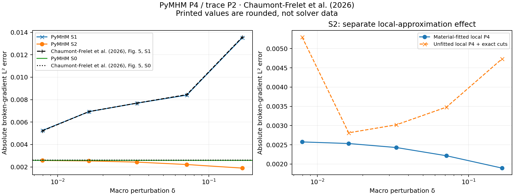
The right panel keeps S2 and the same macro and skeletal spaces, comparing material-fitted versus unfitted local P4 triangles. At \(\delta=1/6\), their gradient errors are 0.00189484 and 0.00473545, respectively. Both use exact material-intersection integration. This is direct evidence that accurate integration and a fitted skeleton alone do not remove local approximation error.
What the remaining S2 difference means
A separately assembled reference solves the stated aligned problem on \(1024\times1024\) squares. Both common interpretations of the article's “piecewise linear” description are checked: bilinear Q1 on each square, and continuous P1 on two triangles per square. Separation in the \(x\) direction reduces these independently assembled systems to tridiagonal systems in \(y\). On grids of 8, 16 and 32 intervals, their nodal solutions agree with independent sparse element assembly within \(4.3\times10^{-16}\).
Since \(a\ge1\), Galerkin orthogonality gives
The first integral uses 8191 odd Fourier modes; the positive omitted energy has an analytical upper bound of \(3.43\times10^{-15}\). The computed energy errors are \(1.74957\times10^{-4}\) for Q1 and \(2.38348\times10^{-4}\) for P1. These are numerical evaluations of the bound, not interval-arithmetic certificates. Their margin is ample for the following comparison:
Consequently, replacing the analytical reference by either of these fine Galerkin references can increase the present final S2 error to at most about 0.002134. It cannot explain a published value around 0.00263. The article's fine reference and the analytical reference are different, but that difference alone is quantitatively too small.
The gradient of a continuous interpolant of broken pressure is not the broken gradient used in Figure 5. For example, transferring the same local P4 fields to a global \(1024\times1024\) P1 mesh with averaged incident nodal values gives 0.01001872 for S0 and 0.00496509 for S2. The underlying broken-gradient errors at local refinement eight are 0.00259415 and 0.00189433. Such a transfer resolves pressure jumps into continuous layers and therefore defines a different norm; it cannot explain the printed S0 and S2 values simultaneously. The verification record includes four transfer resolutions and both averaging and first-incident conventions.
A complete Figure 5 reproduction still requires the original macro coordinates, local meshes and polynomial degrees, coefficient quadrature, trace connectivity, raw S2 values, and the executable norm-evaluation procedure. Section 6 states that local errors are negligible without giving those local parameters. The institutional software page describes access to the authors' implementations by request; the article and its institutional preprint by Chaumont-Frelet, Paredes and Valentin (2023) do not identify a Figure 5 input archive. Inspection of MSL Core, MSL MHM and the separately supplied MHMUN-RAD source does not establish which implementation generated this figure. The present evidence therefore establishes the stated equations and excludes two concrete explanations; it does not establish an error in the published curve or identify a unique historical cause. The diagnostic record contains all levels, assembly checks, bounds, source revisions and digests.
Independent native assembly
An independent DOLFINx/UFL construction assembles the same P4 local spaces, piecewise coefficient, source and signed DG-P2 trace functionals, then solves the complete uncondensed saddle system with PETSc/MUMPS. It covers all eleven heterogeneous configurations declared in this study, using the same sixteen macrotriangles and material-fitted local refinement 16. The S2 trace partitions follow the material intersections, while S1 retains its unsplit macrofaces.
The comparison integrates differences of the complete pressure, broken gradient and physical flux fields on the same local triangles. It also verifies the pressure and skeletal coefficients, original full-system equations and the analytical-error norms of each displayed result. Thus the native calculation checks the operator assembly and the global coupling independently of PyMHM's condensation.
| Configuration | Macro-interface offset delta | Full-system unknowns | Relative physical-flux L2 difference |
|---|---|---|---|
| S0 | 0 | 34,404 | 1.450e-12 |
| S1 | 1/126 | 36,540 | 1.058e-12 |
| S2 | 1/126 | 36,561 | 1.131e-12 |
| S1 | 1/62 | 34,444 | 2.002e-12 |
| S2 | 1/62 | 34,465 | 1.935e-12 |
| S1 | 1/30 | 34,468 | 2.058e-12 |
| S2 | 1/30 | 34,489 | 2.002e-12 |
| S1 | 1/14 | 34,532 | 1.153e-12 |
| S2 | 1/14 | 34,553 | 1.150e-12 |
| S1 | 1/6 | 34,660 | 1.584e-12 |
| S2 | 1/6 | 34,681 | 1.486e-12 |
Across these eleven systems, the maximum relative pressure, broken-gradient and physical-flux differences are 1.488e-12, 1.993e-12 and 2.058e-12, respectively. The denominator is the corresponding independent native field norm, without smoothing or projection across material interfaces. The compensated defects of the original complete equations, divided by the physical load norm, are at most 2.845e-12 for the native fields and 8.287e-11 for PyMHM. The analytical-error norms agree between the current fields within 1.839e-14 in absolute value. Each numerical archive retains both pressure fields, both multiplier vectors and their physical mesh coordinates.
The eleven-case native verification record
preserves individual norms, operator-source digests, package builds and the
verified upstream release of FEniCS/DOLFINx 0.9.0.
The application independently assembles the specified case through UFL; it is
not an original Figure-5 application supplied by the article's authors.
These results establish discrete agreement for the declared configuration,
while the unidentified historical local discretization prevents a claim of
literal Figure-5 reproduction. Three smaller r4 configurations are retained
in the additional native record;
the light native regression is tests/test_unfitted_fenics.py.
The smooth problem of §6.1 has a separate full-system verification on the same 16 crisscross macrotriangles, with local P6 on four fine triangles per macroelement and discontinuous traces of degree zero or one on one or two segments per face. Across these four systems, native UFL and PyMHM pressure coefficients differ by at most \(4.31\times10^{-14}\), trace coefficients by \(2.86\times10^{-13}\), and the native relative residual is below \(6.29\times10^{-14}\). With one segment, the independently assembled P0 and P1 trace solutions coincide to \(2.60\times10^{-14}\) in their pressure coefficients; both have absolute broken-gradient error 1.7935786992. With two segments, that error remains 1.7935786992 for P0 and decreases to 0.2320020704 for P1. The smooth native record identifies every operator, quadrature and source digest. This establishes the discrete symmetry and global coupling for these specified spaces; it does not identify the article's unspecified local resolution.
The independent MSL MHM controls use the same sine forcing, homogeneous weak Dirichlet data and sixteen crisscross macrotriangles, with continuous local P1 pressures. The record identifies the executed msl_mhm, msl_cg and msl_core revisions and their source URLs. It compares every pressure node and raw-flux triangle by physical coordinates. The largest differences between codes are \(2.14\times10^{-14}\) in nodal pressure and \(1.64\times10^{-12}\) in a raw-flux component. Independent reintegration of the exported fields agrees with MSL's gradient-error norm to \(1.56\times10^{-15}\) in absolute value.
| Local refinement \(r\) | Trace degree \(\ell\) | Segments per macroface | Absolute gradient error |
|---|---|---|---|
| 8 | 0 | 1 | 1.816304932 |
| 16 | 0 | 1 | 1.799324401 |
| 32 | 0 | 1 | 1.795023635 |
| 32 | 0 | 2 | 1.795023635 |
| 32 | 1 | 1 | 1.795023635 |
| 32 | 1 | 2 | 0.262056788 |
Thus local refinement preserves the coarse-trace error plateau, and the three coarse trace choices at \(r=32\) give the same norm to rounding. Refining both trace degree and segmentation reduces that error. These local-P1 controls are distinct from the local-P6 UFL checks and the high-order local-resolution campaign. They establish agreement of matching discrete problems across codes; they do not identify an unavailable historical driver or reproduce the plotted Figure-2 values.
Flux, transmission and balance
At \(\delta=1/6\), the errors and macro balances are:
| Setting | Pressure error \(E_p\) | Gradient error \(E_g\) | Energy error \(E_A\) | Maximum macro balance defect |
|---|---|---|---|---|
| S0 | 9.07627e−5 | 2.59414e−3 | 2.83051e−3 | 1.735e−16 |
| S1 | 4.37023e−4 | 1.35360e−2 | 1.59734e−2 | 1.804e−16 |
| S2 | 6.12546e−5 | 1.89484e−3 | 2.11294e−3 | 1.527e−16 |
The balance uses the conservative skeletal flux: total outward flux minus the integral of the source on each macrocell. Across all 33 fitted-local solves, its largest absolute defect is below \(2.0\times10^{-16}\). This verifies the discrete constant-test equations, not pointwise continuity of the raw primal flux or accuracy of the pressure. S1 satisfies this balance while having substantially larger approximation errors.
The displayed flux is \(q_h=-a\nabla p_h\), evaluated independently on each fine triangle. Material values at interface samples are selected from the incident triangle; opposite traces are not averaged. The plots use the existing P4 gradient samples and preserve separate fine-cell connectivity. Their linear color interpolation is only a display device, not the error quadrature used in the tables.
On the horizontal material interface, the exact normal component \(q_y\) is continuous; the tangential component \(q_x\) generally jumps because pressure has a continuous tangential derivative but the coefficient changes by ten. The black profile ticks mark actual macroface intersections. The numerical curves retain both material traces and every sampled discrepancy. Raw primal flux is not asserted to satisfy exact pointwise transmission or fine-cell mass conservation; those stronger properties require an appropriate H(div) mixed solution or flux reconstruction.
For these archived samples, the largest absolute normal-flux discrepancies are 0.04598, 0.57248 and 0.04787 for S0, S1 and S2. These are sampled maxima, not integrated errors or certified suprema. Pressure minima are respectively −0.001345, −0.004728 and −0.001152: the formulation imposes boundary data weakly and does not enforce a discrete maximum principle. The improved S2 norms and transmission profiles therefore do not imply exact pointwise positivity or elimination of every local overshoot.
Smooth h/p refinement and material contrast
Section 6.1 uses \(a=1\) and the manufactured solution
The macro mesh has sixteen crisscross triangles and homogeneous weak Dirichlet data. The trace sweeps retain the article's degree and segmentation: \(\ell=0,1,2,3\) with \(H=\mathcal H/2^j\), \(j=0,\ldots,5\), and \(\ell=0,\ldots,4\) with one, two or four segments per macroface; \(\mathcal H=1/2\). The sixteen selected macrotriangles have diameter \(1/2\); their 28 distinct faces comprise twelve edges of length \(1/2\) and sixteen diagonals of length \(\sqrt{2}/4\). Dividing every face into \(s=2^j\) equal segments therefore gives maximum subface length \(H=1/(2s)\) and minimum length \(\sqrt{2}/(4s)\), rather than one common physical length for all faces. This follows the repeated-face-bisection construction in Section 6.1 and the macro diameter specified in the Figure-2 caption. Section 3.2 distinguishes the characteristic skeletal size \(H\) from each actual local diameter \(H_D\).
The selected local pressures are continuous P8 on uniform triangular refinements 16, 24 and 32. Those local discretizations are declared controls, since the article does not provide its numerical local degree or mesh. Error integration uses orders 11 and 13.
The labels P8/r32 and ell3/s32 describe independent spaces. P8 is
the pressure polynomial degree on each fine triangle; r32 divides each
original macro edge into 32 intervals and gives \(32^2=1024\) fine triangles
per macro. ell3 is the multiplier polynomial degree on each skeletal
segment, and s32 divides each original macroface into 32 segments.
Thus ell3/s32 has four polynomial coefficients per segment, or 128 per
original macroface before boundary elimination. Adjacent segments have
independent polynomials and may be discontinuous at their endpoints. Each
interior segment has one shared multiplier, with opposite outward-normal
signs for its two incident macros.
Doubling \(r\) quadruples the fine-triangle count in two dimensions, without
changing the sixteen macrotriangles. Here \(r\) is a subdivision factor,
not a count of successive refinement rounds.
The acquisition driver selects assembly quadrature with --assembly-order
and independent error quadratures with --norm-orders. These orders count Gauss
points per Duffy coordinate on each integration triangle, rather than polynomial
exactness degrees. Darcy applies a local-degree-plus-two floor to volume
integration; boundary data also apply a trace-degree-plus-two floor. Polynomial
trace coupling retains its separate exact degree-dependent rule. The defaults
are local degree plus three for assembly and local degree plus three and five
for norms. Requested and executed assembly orders are recorded separately.
Filename labels such as q13 and nq13-15 denote these quadrature counts;
the physical Darcy field \(q=-a\nabla p\) has a separate meaning.
The integer \(q\) in Theorem 2 of Chaumont-Frelet, Paredes and Valentin (2026) is a regularity index, with \(0\leq q\leq\ell\); it does not denote a numerical Gauss count. The theorem uses exact local solution maps and does not prescribe a finite local polynomial degree or refinement. A finite local space must resolve the skeletal functionals: a nonzero multiplier with zero pairing against every local pressure trace is an algebraic kernel. For local P8, refinement 16 and 32 segments per macroface, the degree-three trace has such a cyclic multiplier kernel. Increasing volume quadrature does not restore uniqueness of that multiplier. With refinement 32 and the same traces, the local coupling has full column rank. This injectivity check is separate from a uniform inf-sup estimate and from local approximation accuracy.
On the full sixteen-macro smooth problem, the admissible P8/r16 and P2/s32
control gives a pressure \(L^2\) difference of \(1.23574\times10^{-11}\) and a
broken-gradient \(L^2\) difference of \(1.10148\times10^{-10}\) between assembly
orders 11 and 13. Integrating these differences with orders 13 and 15 changes
the gradient difference by less than \(2\times10^{-19}\). The exact-gradient
error is approximately \(2.15797\times10^{-7}\), so the assembly increment is
about 0.051% of that error. This measures quadrature sensitivity for this
specified pair; it does not measure the local-refinement error. The lightweight
record examples/results/unfitted/convergence/quadrature-control.json retains
the fields' digests, independent norms, source hashes and coupling-rank checks.
For example, the following fixed-space control acquires both assembly orders with the same independent norm orders, source, macro mesh and trace spaces:
for order in 11 13; do
  pixi run --locked -e test-core python -m examples.unfitted_convergence \
    --study smooth --degree 8 --refinement 32 --maximum-segments 32 \
    --names ell2-s32 ell3-s32 --workers 1 --assembly-order "$order" \
    --norm-orders 13 15 --output build/results/unfitted/quadrature
done
The default assembly order keeps the smooth-p8-r32 filename prefix; selecting
order 13 appends -q13. Independent norm orders 13 and 15 append -nq13-15
to both acquisition and field filenames. Thus these commands produce
smooth-p8-r32-nq13-15.json and smooth-p8-r32-q13-nq13-15.json, with
distinct corresponding field archives. A resumed acquisition requires matching
configuration and numerical-source digests. Compare the physical fields with
examples.unfitted_local_resolution, passing the two explicit archives and
--order 13, then --order 15; an increment in the integrated field differs
from an increment between two exact-error norms. These controls quantify
quadrature sensitivity of the declared local discretization and do not establish
agreement with an unidentified historical local solver.
The field-comparison reader supports monolithic version-2 archives and complete version-2 phase acquisitions. A phase field requires its accompanying acquisition receipt and cell archives, including the executed retained basis and ordered field corrections. Both schemas verify the cardinal nodes, nodal DOF maps and macro orientation before evaluating the independent physical polynomials. The integration uses each archived local geometry and DOF map; compatible dimensions alone do not identify a coefficient vector's basis.
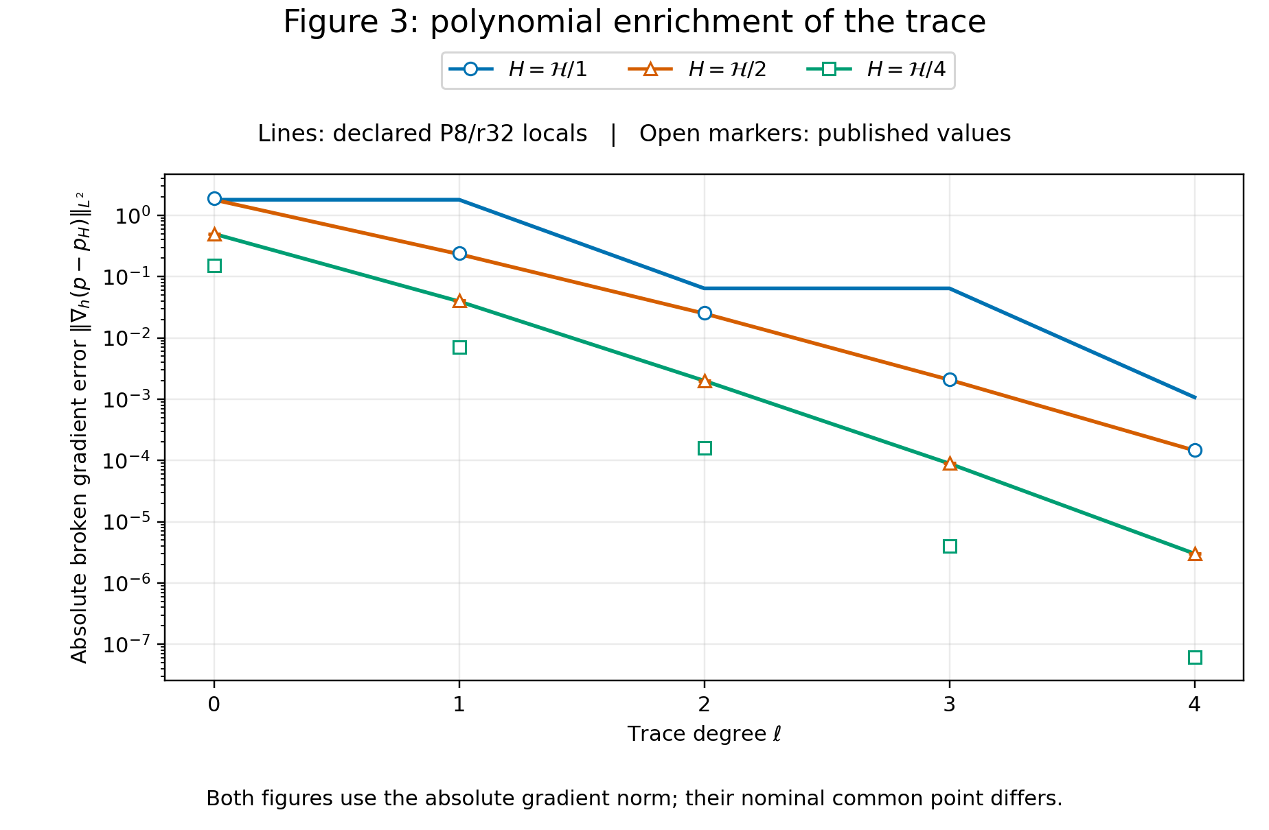
The published-marker record contains 51 values extracted from vector paths in Figures 2, 3 and 7, independently of the PyMHM results. Its intervals propagate one raster pixel at 600 dpi, the vector-coordinate precision and both axis anchors. They measure graphical reading uncertainty, not uncertainty in the original solves.
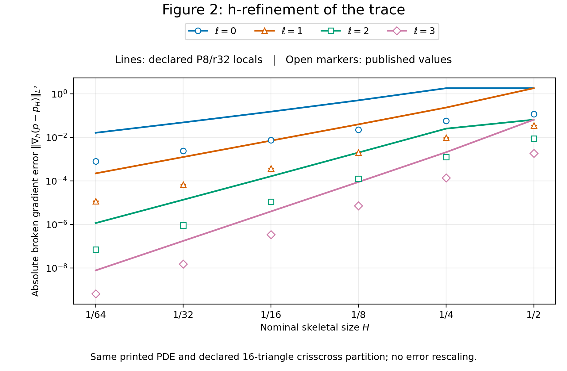
The last three consecutive interval rates of the computed P8/r32 sequence are measured from \(\log(E_j/E_{j+1})/\log(H_j/H_{j+1})\), where \(E_j\) is the absolute broken-gradient error. They approach the \(\ell+3/2\) reference order of the smooth experiment:
| Trace degree | Reference order | s=4 → 8 | s=8 → 16 | s=16 → 32 |
|---|---|---|---|---|
| 0 | 1.5 | 1.729447 | 1.640736 | 1.581800 |
| 1 | 2.5 | 2.491382 | 2.491988 | 2.497230 |
| 2 | 3.5 | 3.623119 | 3.576559 | 3.560654 |
| 3 | 4.5 | 4.492916 | 4.494987 | 4.501484 |
The interval-rate record retains all five intervals and verifies every input field digest. These are rates of the stated finite-dimensional sequence. The local-resolution comparisons below separately quantify the effect of the local meshes; a matching slope alone does not establish negligible local error. The smooth-data rate is not assigned to the discontinuous-material cases.
Figure 2 places its rightmost \(\ell=0\) marker at \(H=0.5\) and absolute gradient error 0.11730413; Figure 3 places the nominal \(\ell=0\), \(H=\mathcal H\) marker at 1.91044. Their ratio is 16.2862. Both captions and axes use the absolute gradient norm, with no squared error or normalization denominator. These nominal labels therefore do not determine a common numerical value. The calculated curves retain the textual PDE and mesh, and both printed marker sets are displayed without rescaling or changing the trace count.
Under that stated bisection construction, all twelve shared nominal \((\ell,H)\) labels in the two figures have disjoint graphical-reading intervals. The table below lists their central values; the complete record retains every interval. The factor \(c=4\) in the Figure-3 legend belongs to its theoretical guide curves, \((cH/(\ell+1))^{\ell+3/2}\), and does not prescribe a normalization of the reported gradient error. These nominal correspondences do not recover the historical input meshes or exclude an unreported change of the abscissa convention. No horizontal or vertical adjustment is fitted to the curves.
| Trace degree | Segments per macroface | Figure 2 | Figure 3 | Figure 3 / Figure 2 |
|---|---|---|---|---|
| 0 | 1 | 0.11730413 | 1.91044 | 16.2862 |
| 0 | 2 | 0.057349594 | 0.49858142 | 8.69372 |
| 0 | 4 | 0.022003928 | 0.15018719 | 6.82547 |
| 1 | 1 | 0.035579612 | 0.24226976 | 6.80923 |
| 1 | 2 | 0.0096668506 | 0.040487773 | 4.18831 |
| 1 | 4 | 0.0020522808 | 0.007110258 | 3.46456 |
| 2 | 1 | 0.0088391497 | 0.02541887 | 2.87571 |
| 2 | 2 | 0.0012325119 | 0.0019961891 | 1.61961 |
| 2 | 4 | 0.00012520915 | 0.00016145653 | 1.28949 |
| 3 | 1 | 0.0018565133 | 0.0021075589 | 1.13522 |
| 3 | 2 | 0.00013608683 | 9.0015936e-05 | 0.66146 |
| 3 | 4 | 7.315596e-06 | 3.9711888e-06 | 0.542839 |
The following independent local-resolution series uses the same specified operator and skeletal partitions at all levels.
| Trace | P8/r16 error | P8/r24 error | P8/r32 error |
|---|---|---|---|
| ell0-s1 | 1.7935787 | 1.7935787 | 1.7935787 |
| ell0-s2 | 1.7935787 | 1.7935787 | 1.7935787 |
| ell1-s1 | 1.7935787 | 1.7935787 | 1.7935787 |
| ell1-s2 | 0.23207961 | 0.23207961 | 0.23207961 |
| ell0-s32 | — | 0.01560128 | 0.016087787 |
| ell1-s32 | — | 0.0002190427 | 0.00022013897 |
| ell2-s32 | — | 8.6666152e-07 | 1.1489802e-06 |
| ell3-s16 | 1.7428698e-07 | 1.7279946e-07 | 1.7471554e-07 |
| ell3-s32 | — | 6.4014269e-09 | 7.7134683e-09 |
| ell4-s4 | 3.0019745e-06 | 3.005129e-06 | 3.0062236e-06 |
The coarse-trace plateau also occurs in the complete UFL saddle systems and independent MSL controls above. Its persistence under local refinement is distinct from the finite local-resolution effects on enriched traces. The following table measures differences between the actual fields on a common physical subdivision, with each trace space held fixed. It does not subtract two scalar exact-error norms.
| Trace | Local refinements | Pressure difference | Broken-gradient difference | Difference / finer exact-gradient error | Order 9/11 gradient change |
|---|---|---|---|---|---|
| ell0-s32 | 24 → 32 | 2.3396165e-06 | 0.0039394028 | 24.4869% | 1.54e-16 |
| ell1-s32 | 24 → 32 | 1.2780033e-08 | 2.1864745e-05 | 9.93225% | 9.13e-16 |
| ell2-s32 | 24 → 32 | 5.4627706e-10 | 7.5682747e-07 | 65.8695% | 3.55e-17 |
| ell3-s32 | 24 → 32 | 2.930455e-12 | 4.2849947e-09 | 55.5521% | 7.19e-15 |
| ell4-s4 | 24 → 32 | 4.8366661e-11 | 8.1114362e-08 | 2.69821% | 6.95e-16 |
| ell3-s16 | 16 → 32 | 9.4724503e-12 | 1.2256108e-08 | 7.01489% | 1.23e-15 |
These observed increments test the selected local resolutions; they are not certified bounds for the exact local problems. In particular, the measured field differences must be compared with the corresponding exact-solution errors; a small change between two scalar error norms does not establish that local approximation errors are negligible. The two independent quadrature orders are preserved in the complete comparison record.
Aligned local-refinement endpoints
Two additional controls retain \(s=32\) and \(\ell=0,1\), and double only the local P8 refinement from \(r=32\) to \(r=64\). Both local meshes resolve the trace breakpoints. The operator, forcing, macro mesh and boundary conditions are identical. The prepared P1 trace contains both target spaces; its restriction preserves the local constant mode.
| Trace | r32 exact-gradient error | r64 exact-gradient error | Pressure difference | Gradient difference | Difference / r64 error | Order 9/11 gradient change |
|---|---|---|---|---|---|---|
| ell0-s32 | 0.016087787 | 0.016116063 | 3.1834621e-07 | 0.00095424449 | 5.92108% | 1.1e-16 |
| ell1-s32 | 0.00022013897 | 0.00022015193 | 7.7936302e-10 | 2.3892456e-06 | 1.08527% | 3.75e-15 |
These differences measure the remaining effect of local resolution at fixed trace space. They are not exact local-error bounds. The endpoint acquisition retains error quadratures 11/13 and field-difference quadratures 9/11. The endpoint record identifies the two physical archives and original-equation checks.
The contrast study retains \(a=a^\star\) below \(y=1/2\) and \(a=1\) above, source one and zero pressure on the exterior. It compares S0 with S2 for \(a^\star=10,10^2,\ldots,10^6\), selecting \(\ell=2\) and \(\delta=1/6\) for S2. Figure 7 does not restate the latter two parameters; this is an explicitly declared control, not identification of a unique historical configuration. Local material-fitted P4 meshes use initial refinements 8 and 16. Their norms use the analytical Fourier solution, orders 7/9 and 1023 odd modes, with a separate 2047-mode check. The reported gradient error is unweighted, so it must not be identified with energy or physical-flux error as the contrast changes.
| Setting | Contrast | P4/r8 gradient error | P4/r16 gradient error | 2047-mode control | Published marker |
|---|---|---|---|---|---|
| S0 | 10 | 0.0025941539 | 0.0025941473 | 0.0025941471 | 0.0026008482 |
| S2 | 10 | 0.0018943281 | 0.0018948416 | 0.0018948413 | 0.0026371064 |
| S0 | 100 | 0.0027850351 | 0.0027850278 | 0.0027850276 | 0.0027916203 |
| S2 | 100 | 0.0018860674 | 0.0018868842 | 0.0018868843 | 0.0039434426 |
| S0 | 1000 | 0.0028114428 | 0.0028114356 | 0.0028114354 | 0.0028180629 |
| S2 | 1000 | 0.0018882466 | 0.0018891045 | 0.0018891046 | 0.0044762816 |
| S0 | 10000 | 0.0028141644 | 0.0028141571 | 0.002814157 | 0.0028207478 |
| S2 | 10000 | 0.0018885022 | 0.0018893643 | 0.0018893644 | 0.0045683013 |
| S0 | 100000 | 0.0028144374 | 0.0028144301 | 0.0028144299 | 0.0028210249 |
| S2 | 100000 | 0.0018885282 | 0.0018893907 | 0.0018893908 | 0.0050523257 |
| S0 | 1000000 | 0.0028144647 | 0.0028144574 | 0.0028144572 | 0.0028210249 |
| S2 | 1000000 | 0.0018885308 | 0.0018893933 | 0.0018893934 | 0.0055104489 |
The same twelve P4/r16 MHM systems are independently assembled with DOLFINx/Basix triangular P4 volume forms and segmented DG-P2 trace forms in UFL. An explicit independent hybrid coupling gives the full saddle system, solved with PETSc/MUMPS. This uses the same physical material, source, boundary data and local and skeletal spaces as each PyMHM calculation. Across contrasts \(10\) through \(10^6\), the maximum relative \(L^2\) differences are \(1.69\times10^{-12}\) for pressure, \(1.98\times10^{-12}\) for its broken gradient and \(6.66\times10^{-10}\) for physical flux. Each denominator is the corresponding independently computed field norm. The largest relative residual of the native full system is \(2.55\times10^{-12}\).
The twelve-case contrast verification record
provides individual field differences, separate evaluations of the PyMHM
solution in both original operators, native-solution residuals and verified
DOLFINx release provenance. The PyMHM runs use
solve_darcy(..., hybrid_refinement_steps=3) with the unchanged original-equation
relative tolerance \(10^{-10}\). Their archives retain complete corrected
pressure fields and physical trace coefficients as portable high/correction/tail
components. The field writer records the cardinal nodal coordinates, local DOF
maps, barycentric multiindices, skeletal subface partitions and normal
orientations. Replay evaluates the complete corrected pressure polynomials on
their original elements and checks the declared cardinal coordinates and
orientation maps; the declared coefficient precision must be available
on the consuming host. The two-pass acquisition also archives its executed
retained matrix, initial fields and ordered physical corrections.
Assembly and norm/export sources
are identified separately. This establishes same-discretization agreement
for the declared S0/S2 cases; the unspecified Figure-7 parameters remain a
limit on literal reproduction of its S2 curve.
The final comparison record retains every signed discrepancy and graphical interval, together with the executed field and source digests. Agreement of individual markers does not establish reproduction of the complete figures.
Analytical and classical references
The numerical norms use an independently derived separation-of-variables solution. For odd \(n\), set \(\kappa_n=n\pi\), \(f_n=4/\kappa_n\), and
On either half-domain, let \(z\) be distance from the horizontal exterior boundary and \(a\) its coefficient. Then
The implementation evaluates equivalent decaying-exponential expressions. Pressure continuity, flux transmission, the forcing series and analytical energy are tested independently. Main norms use 511 odd modes and integration order 8; the three displayed configurations also use 1023 modes and order 10 as an independent sensitivity check.
A separate conforming Q1 assembly uses material-fitted Cartesian grids with 32, 64, 128, 256 and 512 intervals per axis. Its energy errors are 0.00559578, 0.00279890, 0.00139960, 0.000699820 and 0.000349913, computed from Galerkin orthogonality and a 4095-mode analytical energy. This is an independently refined numerical baseline using PyMHM basis kernels, not an independent external code or the article's finest reference mesh.
Recreate the numerical records outside CI and render their figures with:
pixi run --locked -e notebooks python -m examples.unfitted_campaign --collect --fit-locals --refinement 4
pixi run --locked -e notebooks python -m examples.unfitted_campaign --collect --fit-locals --refinement 8
pixi run --locked -e notebooks python -m examples.unfitted_campaign --collect --fit-locals --refinement 16
pixi run --locked -e notebooks python -m examples.unfitted_campaign --fit-locals --refinement 16
pixi run --locked -e notebooks python -m examples.plot_unfitted_validation
The light tests include polynomial moments on material intersections, independent analytical coefficient integrals, complete-operator invariance under sufficient cut quadrature, one-sided material traces and mesh conformity. A fitted P1 transmission patch represents a kinked pressure exactly with continuous physical normal flux; pressure and flux L2 errors must be below \(2\times10^{-13}\) and \(2\times10^{-12}\), respectively. The analytical series is separately checked for boundary values, transmission, differentiated forcing and its energy integral. The targeted suite can be run with:
pixi run --locked -e test-core python -m pytest -q tests/test_cut_cells.py tests/test_scalar_cut_material.py tests/test_layered_poisson_data.py
The full numerical campaign is separate from CI. The published-value record
examples/results/unfitted/published-figure5.json states the transcription
method, rounded values, article identifier and source digest. The flux replay
records archive digests and explicitly distinguishes sampled diagnostics from
integrated norms. The additional h/p and contrast studies above execute the
printed data with explicit local-resolution controls and compare all
51 extracted markers; the stated configuration ambiguities and numerical
differences prevent a claim of complete historical reproduction.
It validates the stated two-dimensional, two-layer scalar problem and the
material/skeleton operations used for it; it is not a validation of arbitrary
three-dimensional interfaces or an unconditional robustness result.
References
-
Théophile Chaumont-Frelet, Diego Paredes, and Frédéric Valentin (2026). Flux approximation on unfitted meshes and application to multiscale hybrid-mixed methods, Computers & Mathematics with Applications 209, 16–27. DOI: 10.1016/j.camwa.2026.01.016.
-
Théophile Chaumont-Frelet, Diego Paredes, and Frédéric Valentin (2022). Flux approximation on unfitted meshes and application to multiscale hybrid-mixed methods, preprint, HAL version 1, 31 October 2022. HAL: hal-03834748v1.
-
Théophile Chaumont-Frelet, Diego Paredes, and Frédéric Valentin (2023). Flux approximation on unfitted meshes and application to multiscale hybrid-mixed methods. Universidad de Concepción, CI²MA, Preprint 2023-02. Institutional preprint.