Darcy on an original SPE10 layer: a small macro mesh and complete material data

This complete application notebook contains the problem data, local and global equations, implementation and recorded results. For the general workflow, start with the method tutorials.

The main workflow is meshes → spaces → local equations → global balance → assemble → solve → fields and errors. MeshHierarchy associates macro and local meshes; bind_interface and LocalContext own supported numbering, geometric orientation and native coordinate conversions. The mathematical forms, physical trace meaning, local modes and gauge remain explicit in the cells below. Fully manual/custom spaces use the same numerical owners; see the custom-interface notebook.

Build the local/global API explicitly for the complete layer 36 of SPE10 Model 2: all \(60\times220\) material pixels are retained, without cropping, smoothing or contrast clipping. MHM uses a \(6\times11\) macro grid. The classical reference uses a much finer single conforming grid.

The geometry, layer and Darcy boundary data follow Paredes, Valentin and Versieux (2024). Their local refinement is not specified; ours is explicit, so this tutorial does not claim a matched discrete reproduction.

Install pymhm[notebooks,visualization] and the compatible native DOLFINx/UFL backend, then open this notebook with jupyter lab in a writable directory. Physical coefficients, local/global equations and conforming reference forms are declared below. Importable scalar helpers handle physical evaluation, norms, plots and archives. Fine reference solves may need several minutes and substantial memory.

The primal hybrid construction follows Harder, Paredes and Valentin (2013); the material layer and face-based comparison above follow Paredes, Valentin and Versieux (2024).

Field evaluation, norms, plots and executed-array archives use the importable supporting scalar helpers. The physical data and local/global variational equations remain explicit below.

The PyMHM distribution contains only the library. The first cell explicitly downloads a checksum-verified companion archive and prepares the declared data using its local Python helpers. You can inspect these support files in ROOT. Complete studies and historical replay retain their existing opt-in flags.

from pathlib import Path
import os
import sys
from pymhm.io.workspace import workspace_from_archive

# Download verified support files; this operation does not execute them.
COMPANION_URL = "https://ipes-lncc.github.io/pymhm/downloads/1d2ec8b0d25291cfc5e4f3f4165491bc39ff665c3c0d7594dd8b2216d1eeed13/darcy_spe10_layer-companion.zip"
COMPANION_SHA256 = "1d2ec8b0d25291cfc5e4f3f4165491bc39ff665c3c0d7594dd8b2216d1eeed13"
WORKSPACE = Path(
    os.environ.get("PYMHM_WORKSPACE", Path.cwd() / ".pymhm-companions" / COMPANION_SHA256)
)
ROOT = workspace_from_archive(COMPANION_URL, sha256=COMPANION_SHA256, directory=WORKSPACE)
os.environ["PYMHM_WORKSPACE"] = str(ROOT)
if str(ROOT) not in sys.path:
    sys.path.insert(0, str(ROOT))

# Explicitly prepare declared data with the downloaded Python helpers.
from scripts.notebook_reproduction import notebook_workspace

ROOT = notebook_workspace("introduction/darcy_spe10_layer.ipynb", directory=ROOT)
root = ROOT
print("Workspace:", ROOT)


import numpy as np
import matplotlib.pyplot as plt
from dataclasses import dataclass
from functools import partial
from typing import Any
from pymhm import Equation, LocalEquations, assemble, columns
from pymhm import MeshHierarchy, LocalContext, bind_interface, bind_problem
from pymhm.core.equations import compile_form
from pymhm.fem.traces.interval import FaceSpace, SkeletonSpace
from examples.introduction.scalar import (
    dirichlet_solve,
    evaluate_bound_pressure,
    evaluate_qk,
    fine_quad_panel,
    broken_quad_panel,
    fine_line_profile,
    grid_quadrature,
    load_spe10_layer,
    native_scalar_space,
    physical_errors,
    plot_convergence,
    plot_field_panels,
)
import ufl
from pymhm import ExecutionConfig, CartesianMacroMesh
from pymhm.fem.scalar.quadrilateral import qk_space, quadrilateral_operators
from pymhm.fem.scalar.operators import boundary_data
from pymhm.materials.cartesian import CartesianCellField
from matplotlib.collections import LineCollection

Workspace: ./build/docs-restructure/final-workspaces/provenance-final-darcy_spe10_layer-645117d9b6e0

1. Read the unchanged data and verify provenance

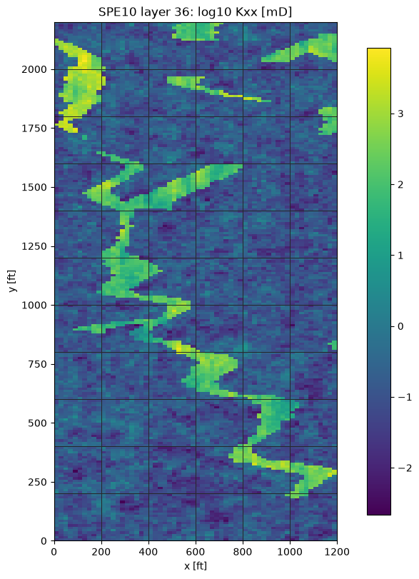
The compact archive preserves the original OPM horizontal entries \(K_{xx},K_{yy}\). The acquisition helper verifies SHA256 and returns CartesianCellField: it selects a declared side at an interface, without averaging. Provenance identifies the project, revision, source URL and axis convention. Coordinates are feet, permeability is mD, and the prescribed pressure difference is dimensionless.

permeability, provenance = load_spe10_layer(ROOT, number=36)
print(
    {
        "source": provenance["repository"],
        "revision": provenance["revision"],
        "layer": provenance["selected_layer"],
        "spacing_ft": permeability.spacing,
        "shape": permeability.values.shape,
        "spectral_contrast": float(
            permeability.values[..., 0, 0].max() / permeability.values[..., 0, 0].min()
        ),
    }
)
macro = CartesianMacroMesh(6, 11, (0.0, 1200.0, 0.0, 2200.0))
pressure_boundary = lambda points: 1 - points[:, 1] / 2200.0
source = 0.0
# K in mD, coordinates in ft; pressure difference is dimensionless in this benchmark.
# Darcy flux therefore has the corresponding benchmark units mD/ft.
local_degree, local_refinement, trace_segments = 1, 80, 16
skeleton = SkeletonSpace(
    macro, tuple(FaceSpace.uniform(1, trace_segments, continuous=True) for _ in macro.faces)
)

{'source': 'https://github.com/OPM/opm-data', 'revision': 'eaa2261683a97027e057c2bc49612ad1c86390b3', 'layer': {'layer_one_based': 36, 'array_index': 35, 'depth_interval_ft': [70, 72], 'kx_range_md': [0.002163, 8412.63], 'phi_range': [1e-07, 0.4], 'kx_equals_ky': True, 'sha256': 'ffe319ce6c126d338a8ad95e497a0121c87e3d7d3eadafb4021ebbe7d3998512', 'file': 'layer-36.npz'}, 'spacing_ft': (np.float64(20.0), np.float64(10.0)), 'shape': (60, 220, 2, 2), 'spectral_contrast': 3889334.2579750344}

2. Same material, operator and boundary data

\[ \begin{aligned} \boldsymbol q&=-K\nabla p,\\ \nabla\cdot\boldsymbol q&=0 \quad\text{in }(0,1200)\times(0,2200),\\ p(x,0)&=1,\qquad p(x,2200)=0,\\ \boldsymbol q\cdot\boldsymbol n&=0 \quad\text{on }x=0\text{ and }x=1200. \end{aligned} \]

pressure_boundary supplies values only to the horizontal Dirichlet faces. Vertical faces have homogeneous physical no-flow data. Every macroelement measures \(200\times200\) ft; material pixels measure \(20\times10\) ft. A local refinement divisible by 20 resolves their interfaces.

Our explicitly integrated local grids align with every material pixel boundary. Gauss integration inside these elements therefore integrates each original constant pixel value. Changing the discretization never changes \(K\). Our local refinement is 80 in each direction, while the macro grid still has only 66 elements. For this fitted grid, a tensor-valued native DG0 coefficient represents each unchanged pixel exactly. The optional alternative operator shown later also supports exact pixel intersections for nonaligned grids.

3. Translate the weak formulation into local and global objects

On each macroelement \(T\), pressure uses a continuous \(Q_k\) fine space. The skeletal multiplier \(\lambda\) is the physical normal Darcy flux in the unique orientation \(\boldsymbol n_F\) of face \(F\). The normal interface binding derives \(s_{TF}=\boldsymbol n_T\cdot\boldsymbol n_F\) from the macroface topology. Write the trace integrals in UFL; LocalContext supplies their basis supports and coefficient maps.

\[ \begin{aligned} a_T(p_T,v)+\langle s_{TF}\lambda,v\rangle_{\partial T}&=(f,v)_T,\\ a_T(p_T,v)&=\int_T K\nabla p_T\cdot\nabla v. \end{aligned} \]

Mathematical term	Code declaration
Local energy and source	`a=inner(Kgrad(p),grad(v))dx`, `L=fvdx` in UFL
Oriented normal-flux pairing	`local.trace_pairings(lambda phi, ds: phivds)`
Constant kernel and physical average	`kernel`, `moments` in `LocalEquations`
Weak pressure continuity	`local.trace_pairings(lambda phi, ds: -phipds, axis="rows")`
Macroface coordinates	`bind_interface(skeleton, convention="normal")` supplies local/global maps

Interior faces have zero pressure-jump moments; Dirichlet faces have prescribed pressure moments. With the declared sign \(C=-B^T\), the additional global right-hand side is

\[ -\sum_T\langle s_{TF}\mu,p_T\rangle_{\partial T} =-\langle\mu,p_D\rangle_{\Gamma_D}. \]

Equation(0, ...) stores this additional global term. One constant mode per macroelement gives the compatibility equation imposing macro conservation. The plotted raw flux \(-K\nabla p_h\) is not an \(H(\mathrm{div})\) reconstruction and is not guaranteed to conserve on every fine cell.

The provider below declares the executable UFL weak forms and each coupling sign. local.native_space owns the native geometry and coefficient convention, while local.trace_pairings binds both interface forms independently. The provider supplies no face DOF indices or nodal permutation. The generic assemble operation owns elimination, assembly and reconstruction; no PDE-specific problem constructor is used.

def ufl_coefficient_source(domain: Any, material: CartesianCellField) -> tuple[Any, Any]:
    """Represent unchanged pixel tensors in native DG0 on a pixel-fitted grid."""
    import basix.ufl
    from dolfinx import fem

    tensor_space = fem.functionspace(
        domain, basix.ufl.element("DG", "quadrilateral", 0, shape=(2, 2))
    )
    coefficient = fem.Function(tensor_space)
    # DG0 interpolation points are cell interiors, so each fitted cell retains its incident pixel.
    coefficient.interpolate(lambda x: material(x[:2].T).reshape(-1, 4).T)
    force = fem.Constant(domain, np.float64(0.0))
    return coefficient, force


@dataclass(frozen=True)
class DarcyLocalProvider:
    """Declare primal Qk UFL energy, physical flux coupling and pressure moments."""

    macro: CartesianMacroMesh
    skeleton: SkeletonSpace
    data: object
    degree: int
    refinement: int
    quadrature_order: int

    def __call__(self, local: LocalContext) -> LocalEquations:
        """Declare K grad(p)·grad(v), f v, oriented normal flux and the constant average."""
        cell, fine = local.cell, local.mesh
        ratios = np.asarray(self.data.spacing) / fine.spacing
        assert np.allclose(ratios, np.round(ratios)) and np.all(ratios >= 1), (
            "DG0 must represent pixels exactly: local cells must fit material boundaries"
        )
        import basix
        import basix.ufl

        element = basix.ufl.element(
            "Lagrange",
            "quadrilateral",
            self.degree,
            lagrange_variant=basix.LagrangeVariant.equispaced,
        )
        binding = local.native_space(element)
        domain, space = binding.mesh, binding.space
        mapping = binding.mapping
        p, v = ufl.TrialFunction(space), ufl.TestFunction(space)
        K, f = ufl_coefficient_source(domain, self.data)
        dx = ufl.Measure(
            "dx", domain=domain, metadata={"quadrature_degree": 2 * self.quadrature_order - 1}
        )
        # These executed UFL forms are the local weak formulation, directly.
        a = ufl.inner(K * ufl.grad(p), ufl.grad(v)) * dx
        load = f * v * dx
        local.field("pressure", binding)
        b = local.trace_pairings(lambda phi, ds: phi * v * ds)
        c = local.trace_pairings(lambda phi, ds: -phi * p * ds, axis="rows")
        area = float(fine.areas.sum())
        return local.equations(
            a=a,
            L=load,
            b=b,
            c=c,
            kernel=np.ones((len(mapping), 1)),
            moments=columns((v / area) * dx),
            metadata=(fine, mapping),
        )

4. Declare global terms and solve MHM

The sidewalls fix the physical normal-flux multiplier to zero. The horizontal pressure boundary contributes the negative right-hand side for \(C=-B^T\). One constant mode is retained per macroelement. Prescribed pressure removes the global gauge.

The visible provider and global declaration define the entire formulation. assemble and system.solve() own the generic condensation, global solution and reconstruction.

Evaluate pressure in its executed coefficient basis

Each named pressure view stores its executed native basis and the corresponding portable Qk coefficient order. evaluate_bound_pressure selects a macrocell and evaluates that view's independent coefficients and physical gradients. The solution coefficients represent pressure; the material tensor \(K\) is applied separately to obtain the physical Darcy flux \(-K\nabla p_h\).

no_flow = {int(face): 0.0 for face in macro.boundary_faces if abs(macro.normals[face, 0]) > 0.5}
boundary, fixed = boundary_data(skeleton, pressure_boundary, no_flow, order=5)
provider = DarcyLocalProvider(macro, skeleton, permeability, local_degree, local_refinement, 5)
hierarchy = MeshHierarchy(
    macro, tuple(macro.submesh(cell, local_refinement) for cell in range(len(macro.cells)))
)
interface = bind_interface(skeleton, convention="normal")
problem = bind_problem(
    hierarchy,
    interface,
    provider,
    global_equation=lambda global_problem: Equation(0, global_problem.trace_load(-boundary)),
    retained=1,
    fixed=fixed,
)
system = assemble(problem, execution=ExecutionConfig("serial", native_threads=1))
solution = system.solve()
pressure_fields = solution.field("pressure")
mhm_fields = tuple(field.portable_coefficients for field in pressure_fields)
mhm_evaluator = partial(evaluate_bound_pressure, macro, pressure_fields)
print(
    {
        "macro_cells": len(macro.cells),
        "local_refinement": local_refinement,
        "trace_degree": 1,
        "trace_segments": trace_segments,
        "global_unknowns": system.matrix.shape[0],
        "fixed_trace_coefficients": len(fixed),
        "largest_local_unknowns": max(len(v) for v in solution.fields),
        "original_equations_relative_residual": solution.raw_residual,
    }
)
# Named fields carry their mesh and executed basis; no index map is needed to evaluate.
first_point = macro.points[macro.cells[0]].mean(axis=0, keepdims=True)
print("First macrocell pressure at its center:", pressure_fields[0].evaluate(first_point))

{'macro_cells': 66, 'local_refinement': 80, 'trace_degree': 1, 'trace_segments': 16, 'global_unknowns': 2599, 'fixed_trace_coefficients': 374, 'largest_local_unknowns': 6561, 'original_equations_relative_residual': 1.8700433007440573e-15}
First macrocell pressure at its center: [0.90553461]

Optional numerical equivalence after the UFL definition

The main formulation above is the executed UFL weak form. Once its operator and coordinate conventions are explicit, quadrilateral_operators provides an alternative assembled representation. The following control verifies equivalence on one local mesh; it does not select the global/local problem or hide its forms. The classical baseline below remains an explicit UFL assembly.

declared = problem.local_provider(0)
fine, mapping = declared.metadata
ufl_a = compile_form(declared.a)
ufl_load = compile_form(declared.L, (len(mapping),))
ready_a, _, ready_load = quadrilateral_operators(
    fine, local_degree, permeability=permeability, source=source, order=provider.quadrature_order
)
operator_defect = np.max(np.abs((ufl_a[mapping][:, mapping] - ready_a).data), initial=0.0)
load_defect = float(np.max(np.abs(ufl_load[mapping] - ready_load), initial=0.0))
print({"UFL_vs_ready_operator_max": float(operator_defect), "UFL_vs_ready_source_max": load_defect})
assert operator_defect < 1e-10 * max(1.0, float(np.max(np.abs(ready_a.data))))
assert load_defect < 1e-10 * max(1.0, float(np.max(np.abs(ready_load))))

{'UFL_vs_ready_operator_max': 1.199040866595169e-14, 'UFL_vs_ready_source_max': 0.0}

5. Conforming Galerkin references and their own uncertainty

There is no analytical solution here. Assemble classical conforming \(Q_3\) on three pixel-aligned grids: \(60\times220\), \(120\times440\) and \(240\times880\). Impose \(p=1\) and \(p=0\) strongly on horizontal boundaries. The sidewalls use the natural zero-flux condition with the same physical Darcy sign.

The fine field is a numerical reference, not an exact solution. Measure differences between successive references in pressure, vector flux and flux energy. High contrast and intersecting material interfaces do not inherit smooth-problem rates.

The common integration grid resolves pixels, local element boundaries and reference boundaries. Norms evaluate each executed coefficient basis directly, rather than interpolating archived images. This is an independent classical assembly sharing basis kernels, not execution of an external paper code.

reference_rows, reference_evaluators, reference_meshes, reference_coefficients = [], [], [], []
for nx, ny in ((60, 220), (120, 440), (240, 880)):
    print(
        f"Assembling conforming Q3 reference {nx} x {ny}; {(3 * nx + 1) * (3 * ny + 1)} coefficients",
        flush=True,
    )
    fine = CartesianMacroMesh(nx, ny, macro.bounds)
    domain, space, mapping = native_scalar_space(fine, 3)
    p, v = ufl.TrialFunction(space), ufl.TestFunction(space)
    K, f = ufl_coefficient_source(domain, permeability)
    dx = ufl.Measure("dx", domain=domain, metadata={"quadrature_degree": 7})
    a_cg = compile_form(ufl.inner(K * ufl.grad(p), ufl.grad(v)) * dx)
    load_cg = compile_form(f * v * dx)
    _, nodes = qk_space(fine, 3)
    exterior = np.flatnonzero(np.isclose(nodes[:, 1], 0.0) | np.isclose(nodes[:, 1], 2200.0))
    coefficients = dirichlet_solve(
        a_cg, load_cg, mapping[exterior], pressure_boundary(nodes[exterior])
    )[mapping]
    reference_evaluators.append(partial(evaluate_qk, fine, 3, coefficients))
    reference_meshes.append(fine)
    reference_coefficients.append(coefficients)
    reference_rows.append({"shape": (nx, ny), "unknowns": len(nodes)})
reference_rows

Assembling conforming Q3 reference 60 x 220; 119641 coefficients

Assembling conforming Q3 reference 120 x 440; 476881 coefficients

Assembling conforming Q3 reference 240 x 880; 1904161 coefficients

[{'shape': (60, 220), 'unknowns': 119641},
 {'shape': (120, 440), 'unknowns': 476881},
 {'shape': (240, 880), 'unknowns': 1904161}]

error_points, error_weights = grid_quadrature(macro.bounds, (480, 880), order=4)
reference_refinement = [
    physical_errors(a, b, permeability, error_points, error_weights)
    for a, b in zip(reference_evaluators[:-1], reference_evaluators[1:])
]
reference = reference_evaluators[-1]
comparison = physical_errors(mhm_evaluator, reference, permeability, error_points, error_weights)
print("Reference refinement:", reference_refinement)
print("MHM versus finest conforming reference:", comparison)
# Refinement evidence is a field measurement, not only a linear residual.
assert reference_refinement[-1]["pressure_L2"] < reference_refinement[0]["pressure_L2"]
assert reference_refinement[-1]["flux_L2"] < reference_refinement[0]["flux_L2"]

Reference refinement: [{'pressure_L2': 0.36075975492633133, 'flux_L2': 0.07688807776026059, 'flux_energy': 0.023104875710699337, 'pressure_relative': 0.00043936012735082316, 'flux_relative': 0.07769816509694663, 'energy_relative': 0.05943437881778285}, {'pressure_L2': 0.17543128502605765, 'flux_L2': 0.05321939892675533, 'flux_energy': 0.014178452433032068, 'pressure_relative': 0.00021361645648628177, 'flux_relative': 0.05387567022744448, 'energy_relative': 0.03649656316095937}]
MHM versus finest conforming reference: {'pressure_L2': 8.635719145906874, 'flux_L2': 0.15414976910511155, 'flux_energy': 0.06575786952330288, 'pressure_relative': 0.010515409055376635, 'flux_relative': 0.1560506562160459, 'energy_relative': 0.16926644496095555}

The plot uses successive reference differences, not errors against an exact solution. The observed slope measures how those increments decrease under simultaneous reference refinement; it does not establish the asymptotic error rate of this heterogeneous problem. Pressure and physical flux can settle at different speeds.

figure = plot_convergence(
    [20.0, 10.0],
    {
        "reference pressure L2 increment": [r["pressure_L2"] for r in reference_refinement],
        "reference Darcy flux L2 increment": [r["flux_L2"] for r in reference_refinement],
    },
)
for axis in figure.axes:
    axis.set_xlabel("Reference x-cell width [ft]")
plt.show()
print(
    "Reference uncertainty/MHM difference ratios:",
    {
        field: reference_refinement[-1][field] / comparison[field]
        for field in ("pressure_L2", "flux_L2", "flux_energy")
    },
)

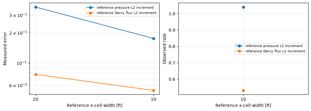
Reference uncertainty/MHM difference ratios: {'pressure_L2': 0.020314612143125094, 'flux_L2': 0.3452447527862732, 'flux_energy': 0.21561605532258907}

6. Fields with the actual macro mesh

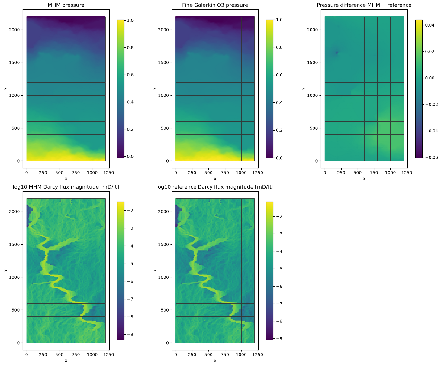
Relate the permeability channels to the physical flux and compare pressure under identical geometry and boundary data. Each panel retains independent macrocell values. The flux fields are raw \(-K\nabla p_h\), not \(H(\mathrm{div})\) reconstructions or averaged multipliers.

Permeability pixels are displayed exactly with nearest-neighbor rendering. The flux-magnitude display uses a logarithmic color scale to show channels across the large contrast; the physical field norms above retain the untransformed vector flux.

Each flux panel samples the actual fine elements independently. The tensor is evaluated at the interior of its pixel-fitted element and applied to that element's own gradient at all four corners. Separate vertices preserve both material-interface and finite-element limits, instead of querying a global coefficient at a shared pixel vertex.

fig, axis = plt.subplots(figsize=(6, 8), layout="constrained")
artist = axis.imshow(
    np.log10(permeability.values[..., 0, 0]).T,
    origin="lower",
    extent=macro.bounds,
    interpolation="nearest",
    aspect="equal",
)
axis.add_collection(LineCollection(macro.points[macro.faces], colors="0.15", linewidths=0.7))
axis.set(title="SPE10 layer 36: log10 Kxx [mD]", xlabel="x [ft]", ylabel="y [ft]")
fig.colorbar(artist, ax=axis, shrink=0.9)
plt.show()

mhm_pressure = broken_quad_panel(system, solution, local_degree, permeability, "pressure")
reference_pressure = fine_quad_panel(
    reference_meshes[-1], 3, reference_coefficients[-1], permeability, "pressure"
)
pressure_difference = (*mhm_pressure[:2], mhm_pressure[2] - reference(mhm_pressure[0])[0])
mhm_flux = broken_quad_panel(system, solution, local_degree, permeability, "flux_magnitude")
reference_flux = fine_quad_panel(
    reference_meshes[-1], 3, reference_coefficients[-1], permeability, "flux_magnitude"
)
# Display log10(magnitude expressed in mD/ft); physical norms remain untransformed.
mhm_flux = (*mhm_flux[:2], np.log10(np.maximum(mhm_flux[2], 1e-12)))
reference_flux = (*reference_flux[:2], np.log10(np.maximum(reference_flux[2], 1e-12)))
panels = {
    "MHM pressure": mhm_pressure,
    "Fine Galerkin Q3 pressure": reference_pressure,
    "Pressure difference MHM − reference": pressure_difference,
    "log10 MHM Darcy flux magnitude [mD/ft]": mhm_flux,
    "log10 reference Darcy flux magnitude [mD/ft]": reference_flux,
}
plot_field_panels(macro, panels, figsize=(15, 12))
plt.show()

7. Macro conservation and profiles with both interface limits

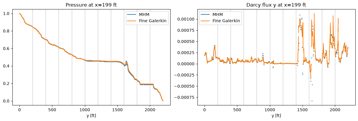
The local constant mode gives \(\int_{\partial T}s_{TF}\lambda=\int_T f=0\). Integrate the oriented skeletal flux in every macroelement to verify this macro balance. This does not prove fine-cell conservation of the raw gradient flux.

Evaluate the \(x=199\) ft profile separately on the eleven macro intervals. Preserve both interface limits, and mark macroface crossings with vertical lines. The profile uses each explicitly selected fine element and its constant incident tensor. It retains both endpoint limits with disconnected line segments, so neither material jumps nor macroface traces are averaged.

macro_balance = []
for cell in range(len(macro.cells)):
    total = 0.0
    for side, face in enumerate(macro.cell_faces[cell]):
        t, w = skeleton.faces[face].quadrature(5)
        normal_flux = skeleton.faces[face].evaluate(t) @ solution.trace[skeleton.dofs(int(face))]
        total += macro.signs[cell, side] * macro.lengths[face] * (w @ normal_flux)
    macro_balance.append(total)
print("Maximum integrated macro imbalance:", float(np.max(np.abs(macro_balance))))
fig, axes = plt.subplots(1, 2, figsize=(12, 4), constrained_layout=True)
for row in range(11):
    field = pressure_fields[row * 6]
    y, p, qy = fine_line_profile(
        field.mesh, local_degree, field.portable_coefficients, permeability, 199.0
    )
    axes[0].plot(y, p, color="C0", label="MHM" if row == 0 else None)
    axes[1].plot(y, qy, color="C0", label="MHM" if row == 0 else None)
y, pref, qref = fine_line_profile(
    reference_meshes[-1], 3, reference_coefficients[-1], permeability, 199.0
)
axes[0].plot(y, pref, color="C1", label="Fine Galerkin")
axes[1].plot(y, qref, color="C1", label="Fine Galerkin")
for ax, title in zip(axes, ("Pressure at x=199 ft", "Darcy flux y at x=199 ft")):
    for y_face in range(200, 2200, 200):
        ax.axvline(y_face, color="0.7", lw=0.7)
    ax.set_xlabel("y [ft]")
    ax.set_title(title)
    ax.legend()
plt.show()

Maximum integrated macro imbalance: 1.6522272439090102e-10

8. What this reference comparison supports

Successive reference differences quantify baseline resolution. Compare them with MHM–reference differences: when baseline uncertainty matters for a field norm, refine the reference further. Pressure often settles before physical flux under this contrast; similar pressure plots do not certify flux accuracy.

For the stated discretizations, the finest reference increment is about 5.4% in physical flux, compared with a 15.6% MHM–reference difference. The flux comparison remains limited by reference resolution: this is a difference against a finite approximation, not the true flux error. Pressure is more settled, with a 0.021% reference increment compared with a 1.05% MHM–reference difference. Further reference refinement is required for more precise flux accuracy.

The method uses 66 macroelements and the declared spaces: local \(Q_1\) pressure and a continuous piecewise \(P_1\) trace on each macroface. Increase local_refinement or trace_segments explicitly for further studies, preserving the original material. Do not alter the approximation family solely to fit an image.

Primary data source: OPM/opm-data, SPE10 Model 2. Acquisition prints the exact revision and SHA256. The opening attribution distinguishes the literature problem from a matched reproduction. This notebook executes PyMHM and a separately assembled classical baseline, not an external article implementation.

References

Christopher Harder, Diego Paredes, and Frédéric Valentin (2013). A family of Multiscale Hybrid-Mixed finite element methods for the Darcy equation with rough coefficients, Journal of Computational Physics 245, 107–130. DOI: 10.1016/j.jcp.2013.03.019.
Diego Paredes, Frédéric Valentin, and Henrique M. Versieux (2024). Revisiting the robustness of the multiscale hybrid-mixed method: The face-based strategy, Journal of Computational and Applied Mathematics 436, 115415. DOI: 10.1016/j.cam.2023.115415.

Run this application notebook

View the source notebook or download the notebook, then open it:

python -m pip install 'pymhm[notebooks,visualization]'
jupyter lab darcy_spe10_layer.ipynb

The first cell explicitly downloads a SHA256-verified companion archive. Acquisition does not execute its code. The local support files are inspectable in the printed ROOT directory; the following helper call prepares only the declared inputs. The library distribution contains only pymhm. Notebooks, support code and data are separate downloads. Native UFL forms require the compatible DOLFINx/UFL backend described in the installation guide. A clone and Pixi are unnecessary.

For batch execution, extract the same companion, change to its workspace, and use its local runner with the actual downloaded notebook path:

python -m scripts.run_notebooks /path/to/darcy_spe10_layer.ipynb --timeout 7200

The runner uses the active Python interpreter and writes an executed copy and receipt under build/notebooks/introduction/. Larger data and field archives have documented download links and verified checksums.

The displayed figures and numerical outputs correspond to the retained validated execution of notebook SHA256 073e30fde6cb2d86672a03262c72d9e514f6ca2956f175fdc7045ac9c23075f4 in the publication manifest. Current instructions use the separately downloaded local examples and scripts support modules. Running the current source produces a separate receipt for its actual notebook, support bytes and environment. Timings describe the recorded hardware and solver settings; measure your own environment on an idle machine.