Darcy: thread scaling
This complete application notebook contains the problem data, local and global equations, implementation and recorded results. For the general workflow, start with the method tutorials.
This notebook declares a Darcy discretization through the public equation API, then checks pressure and physical flux against an independently assembled conforming Q1 solution. The default control has 200 × 200 total fine cells. Complete performance campaigns remain explicit and optional.
DATA.period controls the current material, independently derived forcing, reference and physical-flux integration. The complete timing campaign uses its fixed period-0.1 data.
The domain is the unit square, with zero exterior pressure. The multiplier is the oriented normal flux. Fine Q1 pressures are conforming inside each macrocell; each macroface carries continuous piecewise P1 functions on four segments. The local kernel is the constant function. Physical volume moments select zero-mean source and trace responses.
Here \(p_K\) and \(\lambda\) are coefficient vectors in the local pressure and skeletal bases; \(K\) is the material coefficient. Their basis expansions define the pressure and normal flux fields.
The global system retains one pressure constant per macrocell together with the multiplier. The physical flux below is the broken gradient field \(-K\nabla p_h\); the figures do not assert fine-cell H(div) conservation.
The PyMHM distribution contains only the library. The first cell explicitly
downloads a checksum-verified companion archive and prepares the declared data
using its local Python helpers. You can inspect these support files in ROOT.
Complete studies and historical replay retain their existing opt-in flags.
from pathlib import Path
import os
import sys
from pymhm.io.workspace import workspace_from_archive

# Download verified support files; this operation does not execute them.
COMPANION_URL = "https://ipes-lncc.github.io/pymhm/downloads/cfdd0600c19117937babd3d6ca80c9b96efa1ae23dd7eccc7f5c100d384b797a/darcy_parallel_scalability-companion.zip"
COMPANION_SHA256 = "cfdd0600c19117937babd3d6ca80c9b96efa1ae23dd7eccc7f5c100d384b797a"
WORKSPACE = Path(
    os.environ.get("PYMHM_WORKSPACE", Path.cwd() / ".pymhm-companions" / COMPANION_SHA256)
)
ROOT = workspace_from_archive(COMPANION_URL, sha256=COMPANION_SHA256, directory=WORKSPACE)
os.environ["PYMHM_WORKSPACE"] = str(ROOT)
if str(ROOT) not in sys.path:
    sys.path.insert(0, str(ROOT))

# Explicitly prepare declared data with the downloaded Python helpers.
from scripts.notebook_reproduction import notebook_workspace

ROOT = notebook_workspace("introduction/darcy_parallel_scalability.ipynb", directory=ROOT)
root = ROOT
print("Workspace:", ROOT)


import inspect
import numpy as np
from IPython.display import Code, display
from pymhm import MeshHierarchy, bind_interface, bind_problem
from pymhm.core.equations import Equation
from pymhm.core.multiscale import assemble
from pymhm.execution.cpu import ExecutionConfig
from examples.introduction import scaling_forms as forms, scaling_threads as study

DATA = forms.PeriodicDarcyData(period=0.1)
RUN_CAMPAIGN = os.environ.get("PYMHM_RUN_CAMPAIGN", "0") == "1"
Workspace: ./build/docs-restructure/final-workspaces/provenance-final-darcy_parallel_scalability-cc8411f2fd7c
The displayed source is the actual importable local declaration, shared by both 2D scaling notebooks. Importable providers allow the same declaration to run under threads or cross-platform spawn. To change the formulation, edit this provider or pass your own importable callable to bind_problem; no ready Darcy solver is called.
The UFL declaration shows the weak volume and trace forms. The numerical provider uses the same public assembly operations; the native equivalence check includes all normal orientations and mean moments.
display(Code(inspect.getsource(forms.define_ufl_local_equations), language="python"))
display(Code(inspect.getsource(forms.LocalProvider.__call__), language="python"))
forms.verify_source(DATA)
form_checks = study.verify_forms(DATA)
print(form_checks)
def define_ufl_local_equations(
    local: LocalContext, data: PeriodicDarcyData = DEFAULT_DATA
) -> LocalEquations:
    """Write local volume and interface forms without numbering or orientation code."""
    binding = local.native_space(degree=1)
    domain, V = binding.mesh, binding.space
    p, v = ufl.TrialFunction(V), ufl.TestFunction(V)
    x, y = ufl.SpatialCoordinate(domain)
    frequency = 2 * np.pi / data.period
    K = ufl.exp(ufl.sin(frequency * x) * ufl.sin(frequency * y))
    p_exact = ufl.sin(np.pi * x) * ufl.sin(np.pi * y)
    grad_K = (
        frequency
        * K
        * ufl.as_vector(
            (
                ufl.cos(frequency * x) * ufl.sin(frequency * y),
                ufl.sin(frequency * x) * ufl.cos(frequency * y),
            )
        )
    )
    grad_exact = np.pi * ufl.as_vector(
        (ufl.cos(np.pi * x) * ufl.sin(np.pi * y), ufl.sin(np.pi * x) * ufl.cos(np.pi * y))
    )
    f = 2 * np.pi**2 * K * p_exact - ufl.dot(grad_K, grad_exact)
    dx = ufl.Measure("dx", domain=domain, metadata={"quadrature_degree": 6})
    a = K * ufl.inner(ufl.grad(p), ufl.grad(v)) * dx
    L = f * v * dx

    # Write both mathematical pairings explicitly. The interface adapter supplies
    # their basis, geometric support and outward-normal transport.
    b = local.trace_pairings(lambda phi, ds: phi * v * ds)
    c = local.trace_pairings(lambda phi, ds: phi * p * ds, axis="rows")
    return local.equations(
        a=a,
        L=L,
        b=b,
        c=c,
        kernel=np.ones((len(binding.mapping), 1)),
        moments=columns(v * dx),
        metadata={"native_to_cartesian": np.argsort(binding.mapping)},
    )
    def __call__(self, local: LocalContext) -> LocalEquations:
        """Declare A p+B lambda=f and C=B.T with the physical volume mean."""
        cell, fine = local.cell, local.mesh
        A, mass, f = quadrilateral_operators(
            fine,
            1,
            permeability=self.data.permeability,
            source=self.data.source,
            order=self.quadrature_order,
        )
        B = translated_interface(
            self.coupling_template,
            self.template_endpoints,
            self.macro,
            cell,
            self.face_lengths,
            self.face_space,
        )
        constant = np.ones((len(f), 1))
        return local.equations(
            a=A,
            L=f,
            b=B,
            c=B.T,
            coordinates="global",
            kernel=constant,
            moments=mass @ constant,
            metadata={"mesh": fine},
        )
{0: {'stiffness_max_absolute': 6.217248937900877e-15, 'source_max_absolute': 2.5847379792054426e-16, 'trace_max_absolute': 3.642919299551295e-17, 'mean_max_absolute': 9.75781955236954e-19}, 1: {'stiffness_max_absolute': 1.021405182655144e-14, 'source_max_absolute': 6.418476861114186e-16, 'trace_max_absolute': 2.7755575615628914e-17, 'mean_max_absolute': 2.168404344971009e-18}, 2: {'stiffness_max_absolute': 1.2434497875801753e-14, 'source_max_absolute': 6.279698983036042e-16, 'trace_max_absolute': 3.642919299551295e-17, 'mean_max_absolute': 2.0599841277224584e-18}, 3: {'stiffness_max_absolute': 1.4432899320127035e-14, 'source_max_absolute': 7.28583859910259e-16, 'trace_max_absolute': 2.7755575615628914e-17, 'mean_max_absolute': 3.144186300207963e-18}}
Build the hierarchy, bind the normal trace and declare the zero global right-hand side. Only the execution policy changes between the thread and process notebooks.
macro = study.CartesianMacroMesh(10, 10)
face = study.FaceSpace.uniform(1, 4, continuous=True)
skeleton = study.SkeletonSpace(macro, tuple(face for _ in macro.faces))
template, endpoints = forms.refined_interface_template(macro.spacing, 20, face)
provider = forms.LocalProvider(
    macro, skeleton, template, endpoints,
    forms.face_length_snapshot(macro), face, refinement=20, data=DATA,
)
problem = bind_problem(
    MeshHierarchy(macro, provider.local_mesh),
    bind_interface(skeleton, convention="normal"), provider,
    global_equation=Equation(0, 0), retained=1,
)
execution = ExecutionConfig(
    backend="thread", workers=2, native_threads=1, batch_size=2, pipeline=True,
)
system = assemble(problem, execution=execution)
solution = system.solve()
current_mhm = macro, system, solution
assert len(macro.cells) * provider.refinement**2 == 200**2
print({"fine_cells": 200**2, "trace_dofs": problem.trace_size,
       "retained_dofs": len(macro.cells), "relative_residual": solution.residual})
{'fine_cells': 40000, 'trace_dofs': 1100, 'retained_dofs': 100, 'relative_residual': 1.4123990698251368e-16}
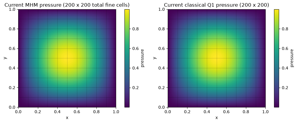
The conforming reference assembles its own Q1 volume operator and strongly eliminates zero exterior pressure. Both represented pressures and physical vector fluxes are integrated on the same partition. Macrofaces remain visible on every spatial panel.
_, current_classical = study.run_classical(200, data=DATA)
current_errors = study.show_control(current_mhm, current_classical, data=DATA)
Numerical output and provenance
Historical campaign provenance: 2026-10-04T20:55:32Z 1427bc29c1a62e3c25fe3d4b541fb285feb19ab7
Archived million-element solver comparison: {
  "classical_LU": {
    "median": 48.290400952100754,
    "minimum": 48.12856928445399,
    "maximum": 48.40943252854049,
    "setup": 1.318651707842946,
    "assembly": 13.781054088845849,
    "solve_reconstruct": 33.308752765879035
  },
  "classical_AMG": {
    "median": 20.8128523491323,
    "minimum": 20.28200477361679,
    "maximum": 20.849384371191263,
    "setup": 1.3477615863084793,
    "assembly": 13.769490350037813,
    "solve_reconstruct": 5.633019220083952
  },
  "thread_MHM": {
    "1": {
      "median": 70.01656742207706,
      "minimum": 69.6620128788054,
      "maximum": 71.37420281767845,
      "setup": 0.6530422940850258,
      "assembly": 69.25675530731678,
      "solve_reconstruct": 0.12755713798105717,
      "strong_speedup": 1.0,
      "strong_efficiency": 1.0,
      "ratio_vs_classical_LU": 0.689699634387878,
      "ratio_vs_classical_AMG": 0.29725610831029914,
      "ratio_vs_fastest_classical": 0.29725610831029914
    },
    "4": {
      "median": 38.20264050364494,
      "minimum": 35.87250446528196,
      "maximum": 38.65109939314425,
      "setup": 0.8551607523113489,
      "assembly": 37.205242693424225,
      "solve_reconstruct": 0.13392465934157372,
      "strong_speedup": 1.8327677484857814,
      "strong_efficiency": 0.45819193712144535,
      "ratio_vs_classical_LU": 1.2640592460485376,
      "ratio_vs_classical_AMG": 0.5448014083515125,
      "ratio_vs_fastest_classical": 0.5448014083515125
    },
    "8": {
      "median": 32.95143252797425,
      "minimum": 32.377874759957194,
      "maximum": 34.575192507356405,
      "setup": 0.8701289687305689,
      "assembly": 31.937516044825315,
      "solve_reconstruct": 0.1476131696254015,
      "strong_speedup": 2.124841381710377,
      "strong_efficiency": 0.26560517271379713,
      "ratio_vs_classical_LU": 1.4655023240978804,
      "ratio_vs_classical_AMG": 0.6316220799039054,
      "ratio_vs_fastest_classical": 0.6316220799039054
    },
    "16": {
      "median": 38.475135535001755,
      "minimum": 38.219250006601214,
      "maximum": 40.25698798522353,
      "setup": 0.6391503289341927,
      "assembly": 37.470310747623444,
      "solve_reconstruct": 0.13368543051183224,
      "strong_speedup": 1.819787414611738,
      "strong_efficiency": 0.11373671341323363,
      "ratio_vs_classical_LU": 1.2551067145213775,
      "ratio_vs_classical_AMG": 0.5409429248195461,
      "ratio_vs_fastest_classical": 0.5409429248195461
    }
  }
}
Current 200 x 200 physical-field control: {
  "MHM": {
    "pressure_L2": 1.2203901833006513e-05,
    "flux_L2": 0.012719053261234495
  },
  "classical": {
    "pressure_L2": 1.2192433581085124e-05,
    "flux_L2": 0.012718368057784214
  },
  "MHM_to_classical": {
    "pressure_L2": 3.7150649141577565e-07,
    "flux_L2": 0.00013204874657346365
  }
}
Current reduced-equation relative residual: 1.4123990698251368e-16
Historical artifacts absent from this checkout: []
The current numerical control above is independent of these historical timings.
Available historical campaign figures (original revision retained above):
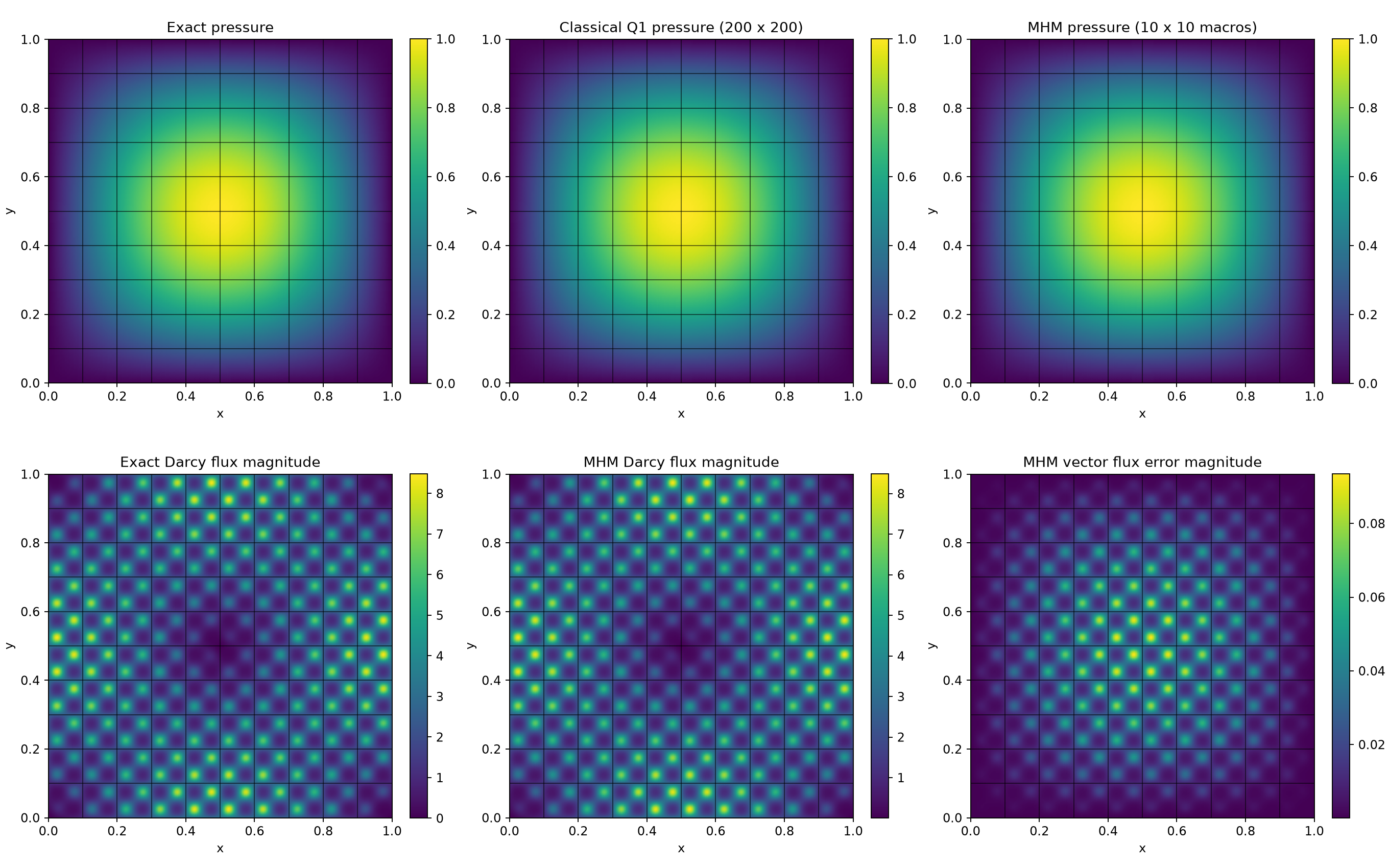
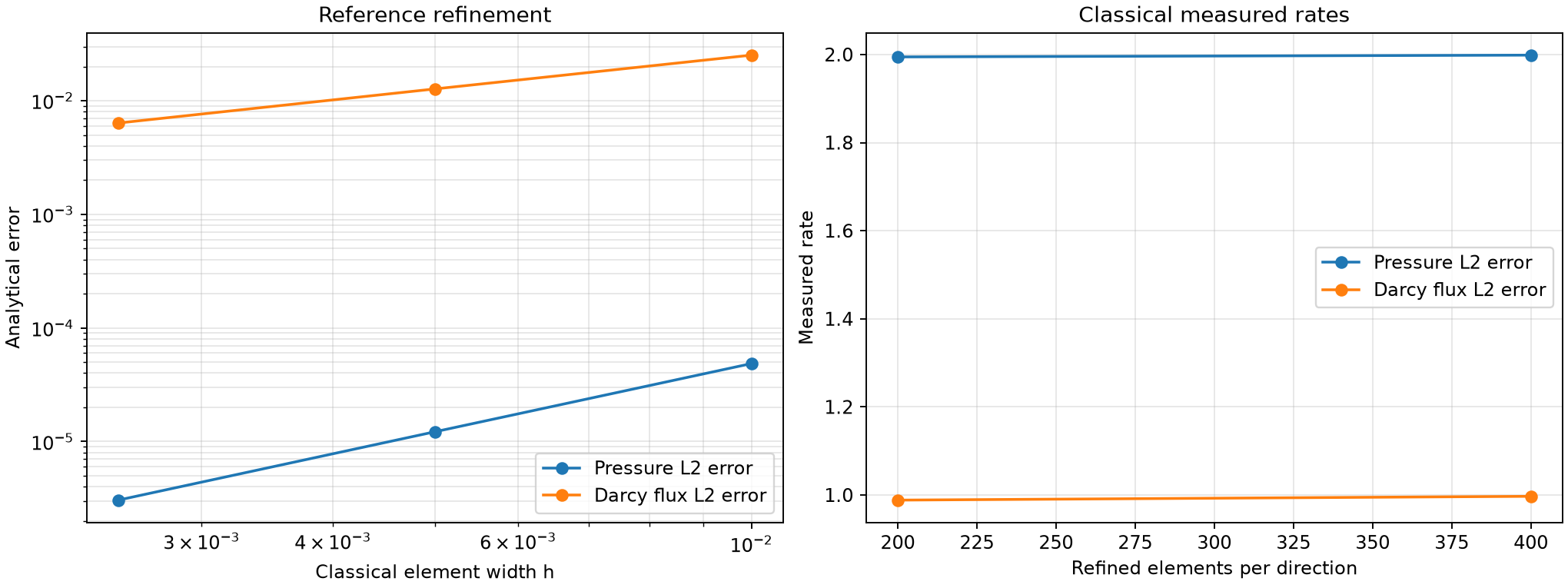
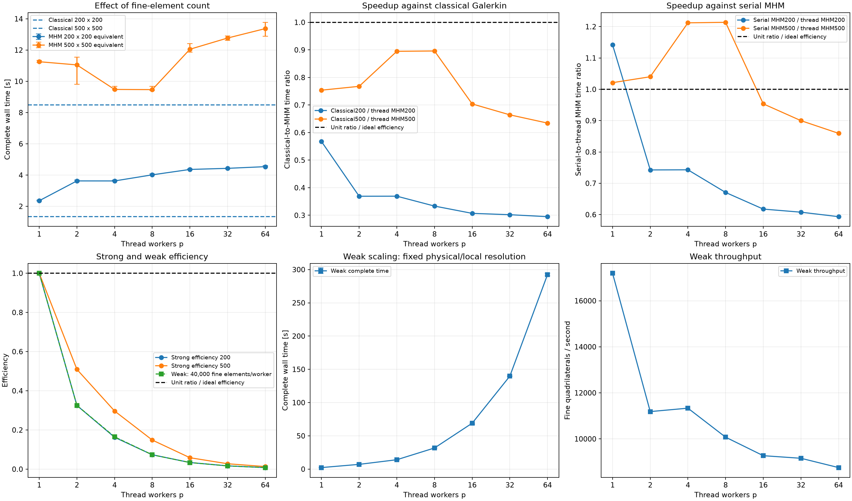
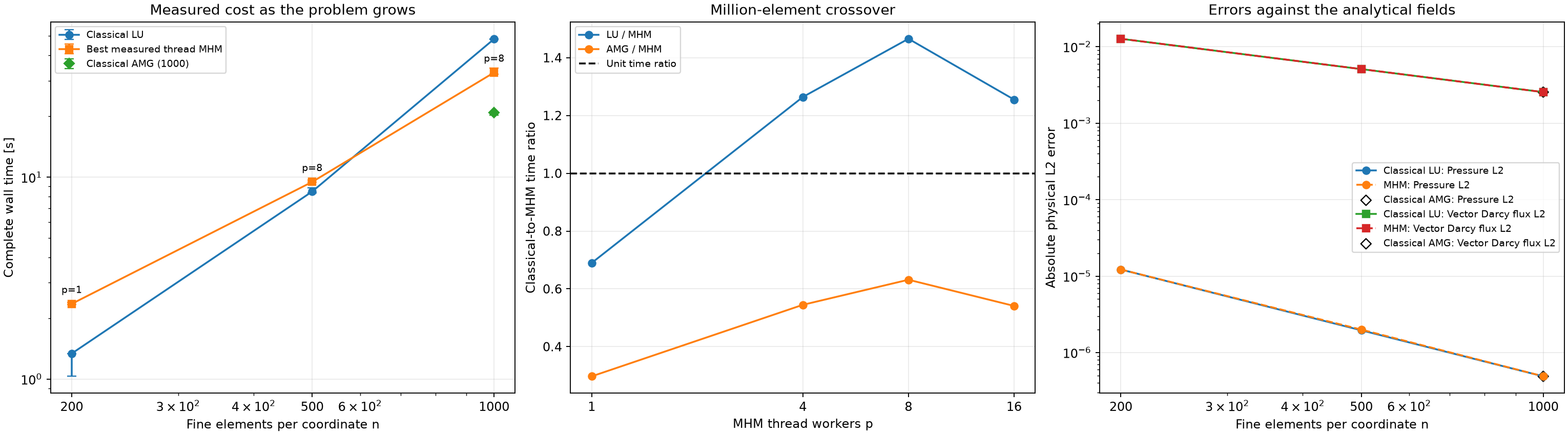
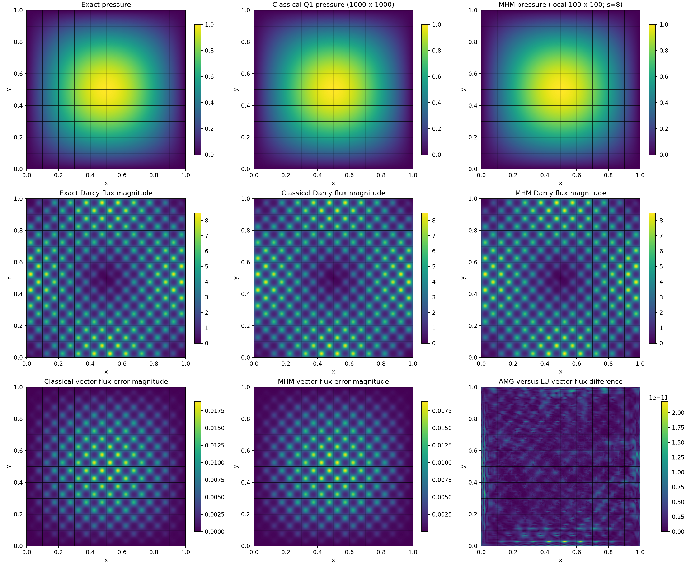
The helper owns timing boundaries, CPU/resource checks, independent norm integration, coefficient/basis archives and plotting. Current controls are shown separately from historical measurements. Each historical record retains its original revision and machine; absent original images are reported explicitly.
Set PYMHM_RUN_CAMPAIGN=1 before execution, or call study.run_campaign() explicitly, to acquire the complete 200/500/1000-axis strong, weak and crossover studies. These campaigns are expensive, require the declared CPU capacity and include fresh worker startup, data transfer, synchronization, global solve and reconstruction. Their source is in the importable scaling helpers.
Run this application notebook
View the source notebook or download the notebook, then open it:
The first cell explicitly downloads a SHA256-verified companion archive. Acquisition does not execute its code. The local support files are inspectable in the printed ROOT directory; the following helper call prepares only the declared inputs. The library distribution contains only pymhm. Notebooks, support code and data are separate downloads. Native UFL forms require the compatible DOLFINx/UFL backend described in the installation guide. A clone and Pixi are unnecessary.
For batch execution, extract the same companion, change to its workspace, and use its local runner with the actual downloaded notebook path:
The runner uses the active Python interpreter and writes an executed copy and receipt under build/notebooks/introduction/. Larger data and field archives have documented download links and verified checksums.
The displayed figures and numerical outputs correspond to the retained validated execution of notebook SHA256 8bcb5fe234b59a269546301a06842a4f932cd217ce7e80208c3ddbd64599335d in the publication manifest. Current instructions use the separately downloaded local examples and scripts support modules. Running the current source produces a separate receipt for its actual notebook, support bytes and environment. Timings describe the recorded hardware and solver settings; measure your own environment on an idle machine.