Maxwell propagation through a photonic device

This case uses the geometry, materials and MHM spaces of Section 6.3 in Lanteri, Paredes, Scheid and Valentin (2018). The local method is central-flux DG Q2 on Cartesian quadrilaterals, coupled through linear tangential traces. The field acquisition includes both coarse meshes from the article and a separately refined classical DG calculation.

Geometry, materials and incident wave

The domain is \([0,10]^2\). The silica device is the union of the rectangles \([3.75,7.5]\times[1.875,8.125]\), \([1.875,3.75]\times[3.125,6.875]\) and \([7.5,9.375]\times[4.375,5.625]\). Fifteen circular inclusions have radius \(0.3125\) and centres in

\[ \begin{aligned} x_c&\in\{4.375,5.625,6.875\},\\ y_c&\in\{2.5,3.75,5,6.25,7.5\}. \end{aligned} \]

Relative permittivity is 1 in air, 1.5 in silica and 3.14 in the inclusions; magnetic permeability is 1. These values are used directly as permittivities, without squaring them as refractive indices. Circular interfaces are sampled by the declared cell quadrature; increasing the quadrature order supplies a separate integration check. The Cartesian field spaces are unchanged.

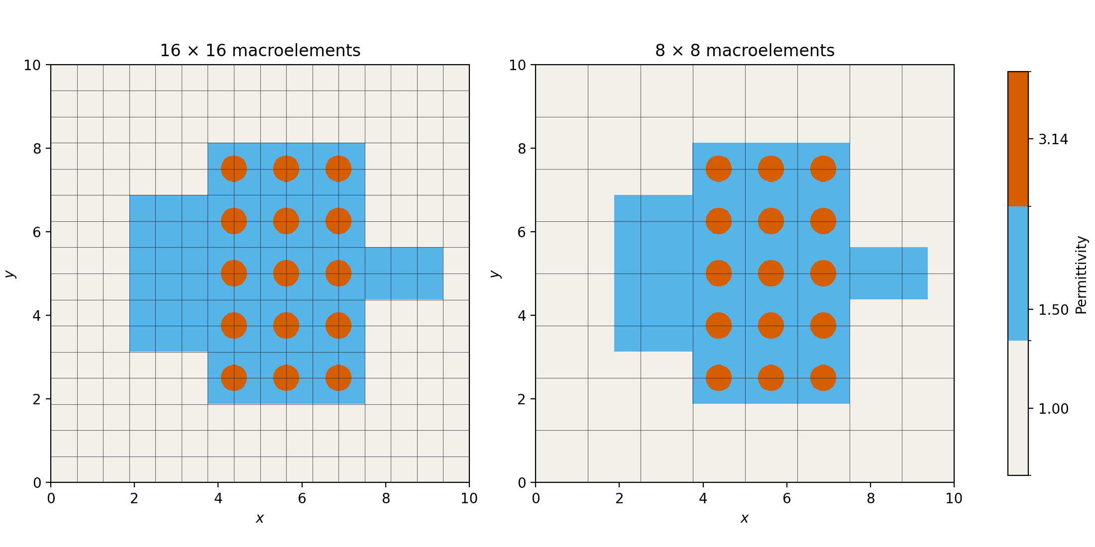
The panels show the same pointwise material distribution. Only the overlaid macro partition changes between the published \(16\times16\) and \(8\times8\) configurations; these are coefficient maps, not electric-field solutions.

The article specifies incident frequency \(f=0.5\), absorbing exterior conditions and final time \(16/\sqrt2\). Phase, amplitude, initial fields and turn-on are not specified sufficiently to reconstruct a unique transient. This comparison declares a causal unit-amplitude wave travelling in the positive \(x\) direction:

\[ \begin{aligned} s&=t-x,\\ E_i(t,x,y)&=\mathbf1_{s\geq0}\sin(\pi s),\\ H_i&=(0,-E_i),\\ E(0)&=H(0)=0,\\ E_z-(H\times n)&=(1-n_x)E_i\\ &\quad\text{on }\partial\Omega. \end{aligned} \]

The identical boundary and initial data are applied to every MHM and classical calculation. These declared data permit a quantitative numerical comparison; they do not establish that the historical incident transient was identical.

Approximation spaces and comparisons

Method	Macro grid	Local fine grid per macro	Tangential trace	Global trace unknowns
MHM, first published configuration	\(16\times16\)	\(8\times8\) Q2 DG	P1 on 8 segments per face	8704
MHM, second published configuration	\(8\times8\)	\(16\times16\) Q2 DG	P1 on 16 segments per face	4608

Both configurations contain the same \(128\times128\) fine quadrilateral partition, with 147456 electric coefficients before condensation. Their published macro step is \(\Delta t=0.01\). Comparisons retain the staggered times \(t_E=11.315\) and \(t_H=11.31\); they do not compare fields at different time coordinates merely because each is the final stored snapshot.

The classical reference uses an original independent matrix-free central-DG Q2 assembly. Fine-grid resolutions, quadrature orders and time steps are varied separately. Its mass, derivative and boundary operators agree with small independently assembled native systems; it does not invoke the MHM local or global operators. Classical DG has no macro partition. Overlays on its plots identify the MHM comparison grid.

Componentwise differences are integrated on the common partition of both grids, using the actual discontinuous Q2 polynomials. Three Gauss points per coordinate integrate their squared differences exactly. The combined norm is

\[ \begin{aligned} \|e\|^2&=\|E_z-E_{z,\mathrm{ref}}\|_{L^2}^2\\ &\quad+\|H_x-H_{x,\mathrm{ref}}\|_{L^2}^2\\ &\quad+\|H_y-H_{y,\mathrm{ref}}\|_{L^2}^2. \end{aligned} \]

It is an unweighted physical field norm. A refined numerical solution is not an exact solution. Its spatial, temporal and material-integration increments determine how precisely it can assess MHM error.

The finest classical calculation has \(1024\times1024\) Q2 cells, 9437184 electric coefficients and \(\Delta t=0.00125\). The retained reference measurements use float64 matrix-free time integration with CuPy on an NVIDIA GeForce RTX 3060. The displayed fields use the same discretization and physical times, acquired on an NVIDIA RTX A5000; their recomputed component norms agree with every percentage in the table below. The field-display record identifies this acquisition separately from the retained measurements. At \(256\times256\), the full CPU and GPU trajectories give a final combined field difference of \(2.95\times10^{-15}\); independent small-matrix checks also cover mass inversion, derivatives and absorbing-boundary forcing. This verifies the two classical implementations of the same discretization.

Calculation	Relative \(E_z\) difference (%)	Relative \(H_x\) difference (%)	Relative \(H_y\) difference (%)	Combined difference (%)
MHM \(16\times16\), \(\Delta t=0.01\)	0.8478	1.3238	0.7385	0.8346
MHM \(8\times8\), \(\Delta t=0.01\)	0.7235	1.2309	0.6320	0.7241
Classical DG \(32\times32\), \(\Delta t=0.01\)	12.2021	22.6121	11.9173	13.0122

All denominators in this table use the finest classical field. Separate controls quantify changes in space, time and material quadrature:

Control	Fixed parameters	Combined relative increment (%)
Classical \(256\to512\) cells per coordinate	\(\Delta t=0.0025\), 12-point material rule	0.3558
Classical \(512\to1024\) cells per coordinate	\(\Delta t=0.00125\), 12-point material rule	0.1270
Classical \(\Delta t:0.0025\to0.00125\)	\(512\times512\) cells, 12-point material rule	0.0800
Classical material rule \(12\to20\)	\(256\times256\) cells, \(\Delta t=0.0025\)	0.0352
MHM \(\Delta t:0.01\to0.005\)	\(16\times16\) macros, published spatial spaces	0.2704
MHM material rule \(20\to28\)	\(16\times16\) macros, \(\Delta t=0.01\)	0.0184

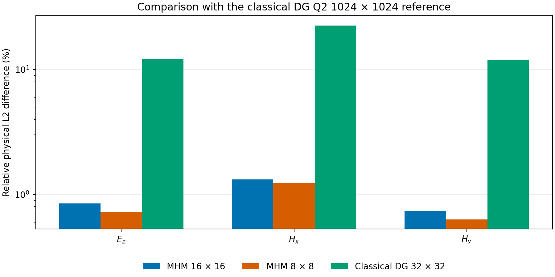
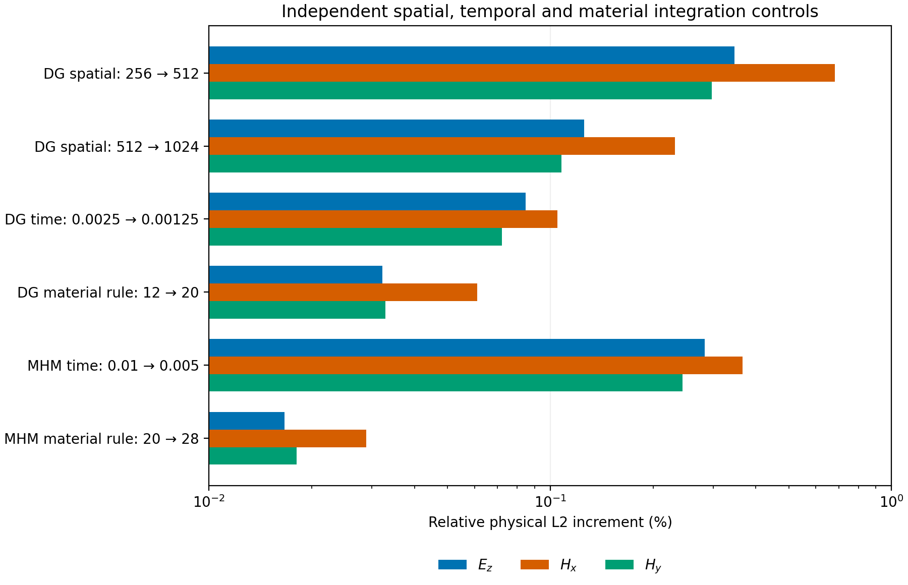
The summary plots display the retained norm measurements at their declared staggered times. Refinement increments compare two numerical calculations; they are not errors against an exact solution. Each increment uses the second configuration as its denominator, at the same staggered physical times. The last spatial increment is about six times smaller than the MHM differences, but remains measurable. These increments are refinement evidence, not rigorous upper bounds on reference error. The temporal control also shows that the published MHM time step contributes to the total discrepancy. No time extrapolation or phase alignment is applied.

This device's independent baseline is central DG. A separately refined conforming transient reference for the same heterogeneous operator and incident data remains an additional physical comparison. The conforming scalar-wave control in the smooth TM tutorial qualifies that analytical cavity problem.

The numerical records retain field digests, integration partitions and componentwise norms: field comparisons, refinement controls and CPU/GPU equivalence.

Fields and one-sided profiles

The panels retain the signed electric and magnetic components. Every row uses a shared field scale. The two MHM difference panels share a scale; the coarse classical DG difference has a separately labelled, larger scale. These images sample the actual cell polynomials at display pixels. The physical norms above use quadrature, rather than those pixels.

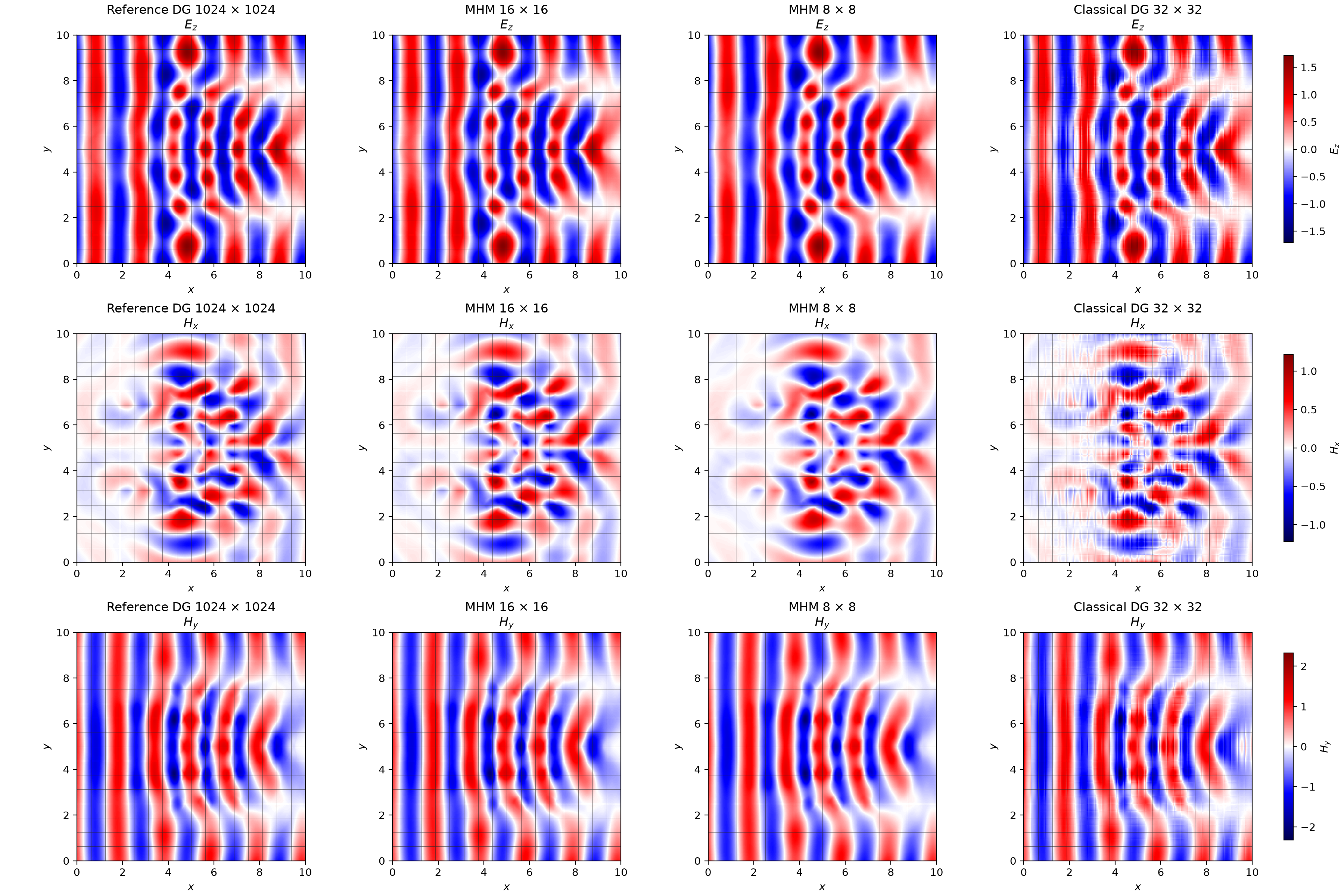
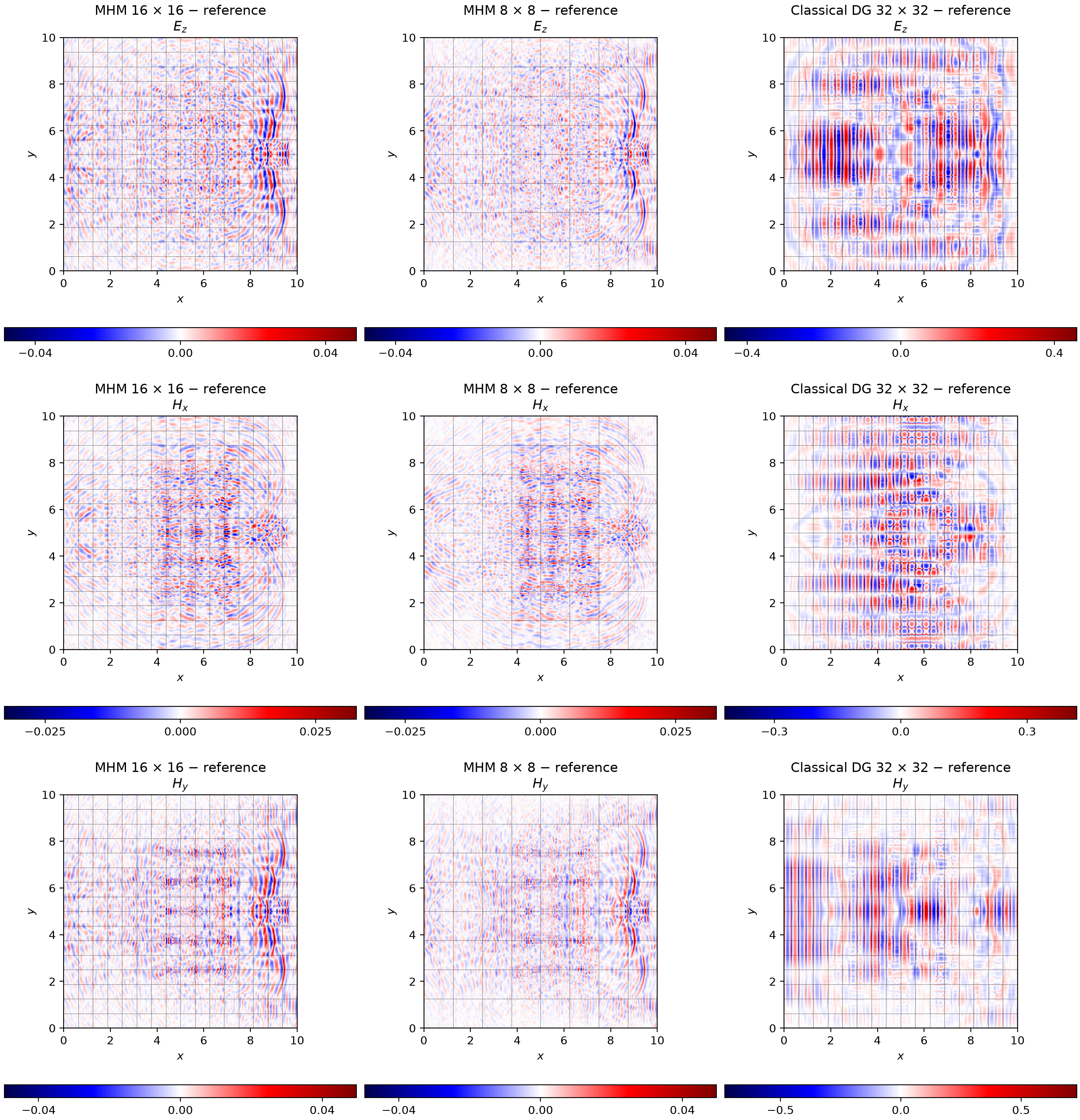
The two horizontal sections avoid mesh vertices and preserve both incident traces at fine-cell boundaries. Dotted lines mark the 16-by-16 macro partition; alternate lines also bound the 8-by-8 partition. The coarse classical DG solution has visible jumps and oscillations that are much smaller in the two MHM solutions.

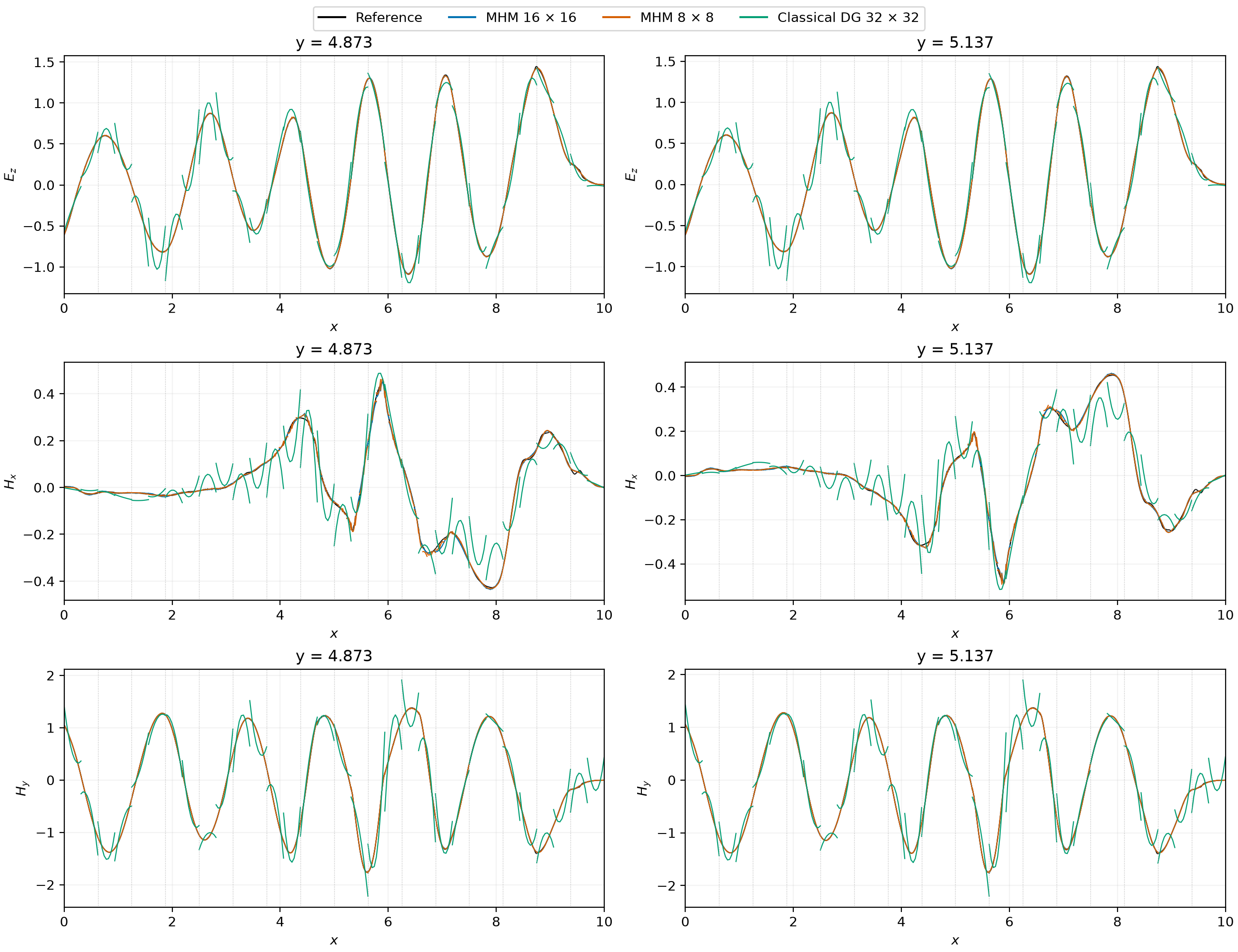
The field-display record identifies the complete coefficient arrays, executed operators, physical times and recomputed component norms used by these maps and profiles. The tabulated comparisons and refinement controls retain their original acquisition digests.

The publication uses the geometry and spaces declared here. Its unspecified incident-wave phase and turn-on prevent an unqualified comparison of the detailed phase and amplitude of the historical images.

pixi run --locked -e test-core python -m examples.maxwell_nanoguide --help
pixi run --locked -e notebooks python -m examples.maxwell_nanoguide_results --records-only

The record-only command regenerates the material and norm-summary figures without rerunning either solver. Regenerating the field maps and profiles with --plot additionally requires the complete Q2 coefficient archives named in the comparison record. Those large field arrays are not bundled with the package or notebook companion.

References

• Stéphane Lanteri, Diego Paredes, Claire Scheid, and Frédéric Valentin (2018). The Multiscale Hybrid-Mixed method for the Maxwell Equations in Heterogeneous Media. Multiscale Modeling & Simulation 16(4) 1648-1683. DOI: 10.1137/16M110037X.