Marmousi acoustic point source
This experiment solves the heterogeneous acoustic problem described in Section 6.4 of Chaumont-Frelet and Valentin (2020) using a declared subdomain of the primary Marmousi II data. The physical domain, frequency, source position and local polynomial families follow that section. The material arrays are an explicitly selected input: they have not been identified with the historical arrays used in Table 6.1.
The image-registration evidence and its numerical record explain this distinction. Similarity of a printed material image does not establish equality of its cellwise coefficients.
Equation, units and material data
Let \(x\) denote horizontal distance and \(z\) depth, both in metres:
The top boundary \(z=0\) has \(p=0\). The other three sides use the outgoing first-order condition
The right-hand side is a unit point-evaluation functional in this equation; there is no calibration to a measured source amplitude. It is assembled at the source point without replacing the Dirac distribution by a Gaussian or a finite well. The complex pressure and both of its real and imaginary parts are retained.
The primary dataset is Martin, Wiley and Marfurt (2006). The input files are the compressional velocity and density SEG-Y records. Their SHA-256 digests are verified before extraction and included in each numerical record.
The original \(13601\times2801\) arrays have spacing 1.25 m. The selected crop has origin \((3395,515)\) m in the primary coordinates and \(2048\times512\) cells of width 5 m. Each material-cell centre coincides with a primary sample. No interpolation or cell averaging is used. The decoded velocity is converted from km/s to m/s, density from g/cm\(^3\) to kg/m\(^3\), and \(\kappa\) is stored in pascals. In this crop,
These values retain the decoded primary samples; rounding here is only for presentation.
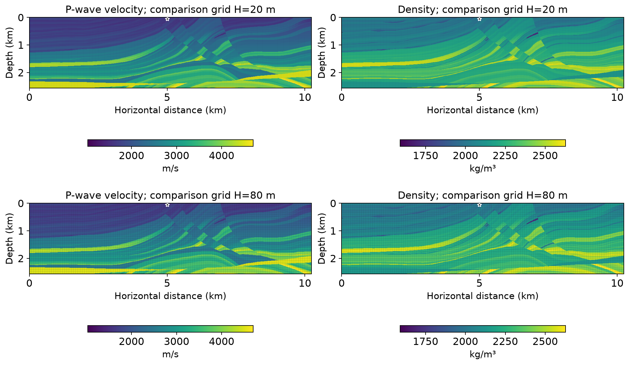
The top row overlays \(H=20\) m macroelements and the bottom row \(H=80\) m macroelements on the same material samples. P-wave velocity is on the left, density on the right, and the star marks the point source.
Classical reference and field verification
The independent classical application uses DOLFINx/UFL on the pixel-conforming southwest-to-northeast triangular mesh. Coefficients are cellwise constant and integrated without averaging across material interfaces. Continuous equispaced \(P_k\) pressures are represented by two real components.
Writing the complex matrix as \(A-\mathrm{i}C\), multiplication of the imaginary test equation by \(-1\) gives the exactly equivalent real system
Five symmetric Ruiz congruences precede the PETSc/MUMPS indefinite \(LDL^\mathsf{T}\) factorization. Acceptance uses the original physical equations after Dirichlet elimination, including the stored coefficients; the equilibration does not change the operator or add damping.
Four polynomial levels have been acquired on the same 2,097,152 triangles:
| Classical space | Complex pressure unknowns | Original-equation residual | Relative native/replayed pressure norm difference |
|---|---|---|---|
| \(P_1\) | 1,051,137 | \(7.06\times10^{-12}\) | \(7.99\times10^{-15}\) |
| \(P_2\) | 4,199,425 | \(2.06\times10^{-11}\) | \(2.69\times10^{-14}\) |
| \(P_3\) | 9,444,865 | \(2.96\times10^{-11}\) | \(1.80\times10^{-14}\) |
| \(P_4\) | 16,787,457 | \(6.15\times10^{-11}\) | \(1.40\times10^{-14}\) |
The native/replayed comparison checks the physical \(L^2\) norm reconstructed from MPI field archives against the independently assembled UFL integral. This is a field-replay verification, not a discretization-error estimate.
Light native checks verify complex constant fields with homogeneous and layered density, the impedance sign, exact Dirichlet values, and a point load against an independently assembled complex conforming matrix. An independent native \(P_3\) constant-field problem also checks the condensed MHM \(Q_3\) solution with nonzero pressure and absorbing boundary data. The postprocessor also recovers non-affine complex \(P_4\) polynomials and nonzero analytical pressure and gradient integrals.
MHM configuration and comparison conventions
The executable MHM configuration uses quadrilateral macroelements, continuous local \(Q_3\) pressures and polynomial conormal traces. For the three macro widths in Table 6.1:
| Macro width \(H\) | Macro grid | Local subdivisions per direction | Local complex pressure unknowns per macro |
|---|---|---|---|
| 20 m | \(512\times128\) | 8 | 625 |
| 40 m | \(256\times64\) | 16 | 2,401 |
| 80 m | \(128\times32\) | 32 | 9,409 |
All three choices have local cell width 2.5 m and resolve every material interface. The driver archives the full local fields; trace degree is a separate input. These are configuration specifications, not assertions that every entry of the published table has been reproduced.
The transcribed published table records all fifteen MHM values from Table 6.1 of the author manuscript, checked against the printed table. For example, \(H=20\) m and trace degree \(\ell=1\) give a published sampled-pressure difference of 2.90%. This number refers to the article's material arrays and reference solution; the present selected crop is a separate, fully specified input.
For a point source on a macro interface, the discrete load is allocated by the incident angular sectors, preserving its total unit strength. Here \(H=20\) m and \(H=40\) m place the source on a vertical macroface: each of its two incident macros receives half of the functional. For \(H=80\) m the source lies inside one macro, which receives the full unit functional. This is the declared broken-space loading convention; the article does not specify that allocation on macro interfaces.
The article's comparison samples a uniform \(513\times129\) grid. This is an unweighted discrete norm, distinct from a physical volume norm. The MHM pressure is broken; a sampling point on an interior macro vertex can have four incident values. The acquisition preserves all four one-sided conventions without averaging them. The historical selection at such points is not stated in the table.
For classical refinement, complex \(L^2\) pressure differences use the complete domain. Gradient, acoustic flux \(q=-\rho^{-1}\nabla p\) and positive graph-norm comparisons instead use the fixed punctured domain
The excluded square has side 50 m, contains the point source, and is exactly aligned with the material pixels at every polynomial level. The graph norm is
The graph norm is not the indefinite Helmholtz bilinear form. Every relative reference increment uses the finer polynomial field as its denominator. With a two-dimensional point source, the continuum pressure does not have finite global \(H^1\) norm. Fixing the excluded physical region keeps these derivative comparisons meaningful as the reference is refined. Neither the global pressure comparison nor the published sampling grid removes points around the source.
The measured consecutive reference increments are:
| Polynomial levels | Global pressure \(L^2\) | Global sampled pressure | Cutout gradient | Cutout acoustic flux | Cutout graph norm |
|---|---|---|---|---|---|
| \(P_1\to P_2\) | 108.610% | 109.129% | 107.139% | 106.907% | 106.914% |
| \(P_2\to P_3\) | 0.398720% | 0.378786% | 0.632198% | 0.638839% | 0.521159% |
| \(P_3\to P_4\) | 0.0785754% | 0.00548487% | 0.0404000% | 0.0412093% | 0.0289480% |
Orders 6 and 8 agree to \(3.1\times10^{-13}\) relative in the integrated differences, including the smallest final increment. The large first increment remains despite small algebraic residuals; the two smaller increments measure the effect of further polynomial resolution on the same material mesh. These are numerical refinement differences, not certified upper bounds on the remaining reference error. The reference-refinement record retains all norms, denominators, data and field digests.
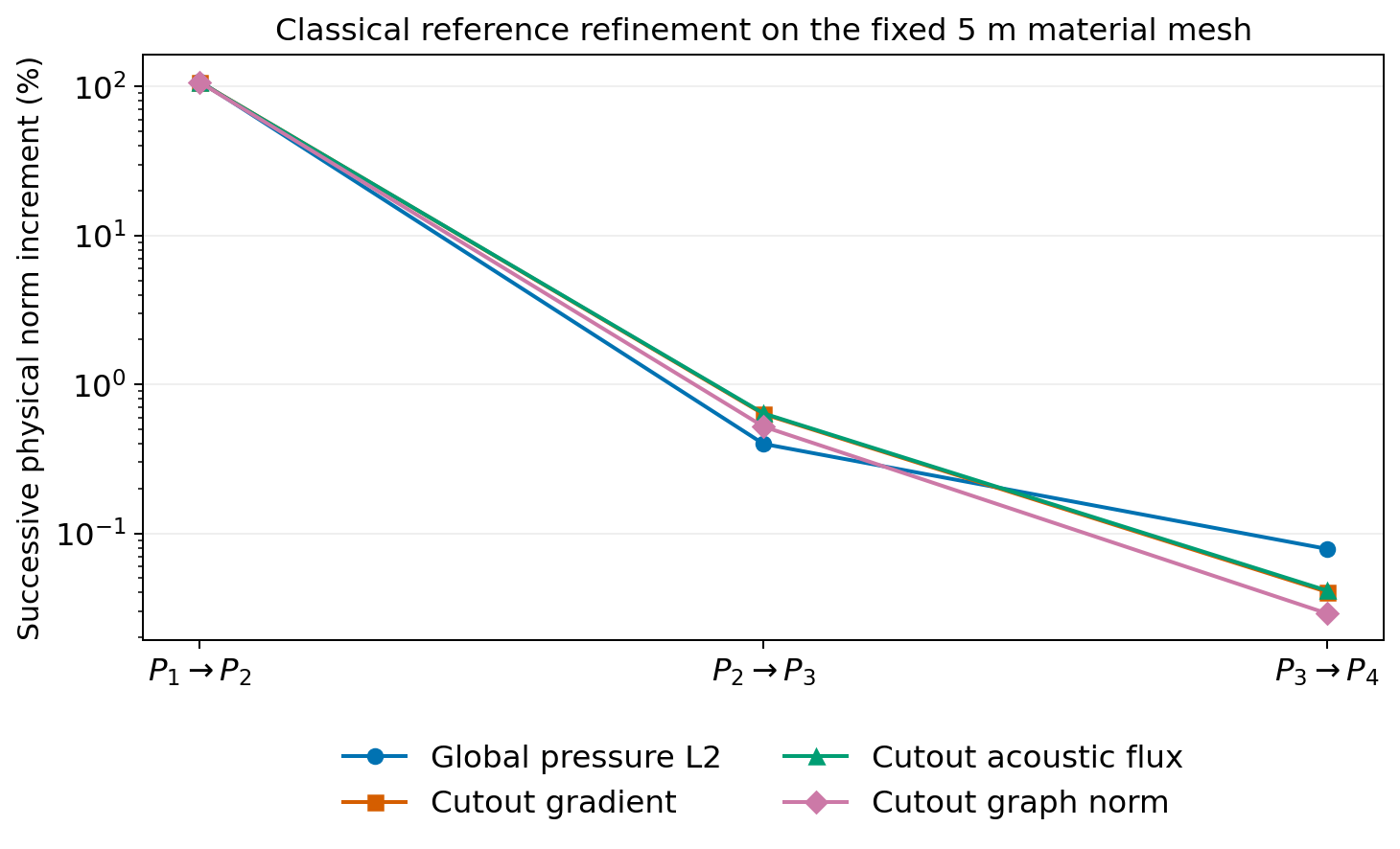
This plot shows polynomial refinement on the fixed material mesh. The derivative norms retain the declared 50-by-50 m square exclusion; the pressure norm remains global. These increments are not errors against an exact solution or an asymptotic mesh-convergence study.
MHM H20 with a linear conormal trace
The acquired \(H=20\) m, \(\ell=1\) configuration has 65,536 quadrilateral macroelements, 625 complex local \(Q_3\) coefficients per macro and 261,888 free complex skeletal unknowns. Its original-equation residual is \(2.84\times10^{-14}\) and its maximum macro balance defect is \(9.41\times10^{-15}\). The independent \(P_4\) baseline above resolves the same declared coefficient arrays, boundary conditions and point functional.
| Difference from classical P4 | Relative value |
|---|---|
| Global pressure \(L^2\) | 2.69345% |
| Cutout gradient | 3.02698% |
| Cutout acoustic flux | 3.03693% |
| Cutout graph norm | 2.87459% |
These differences use 8,388,608 common triangles, resolving both the MHM local rectangles and the classical triangles. Quadrature orders 8 and 10 agree within \(1.2\times10^{-14}\) relative. The pressure norm remains global; all derivative norms use the same fixed physical cutout above. The last classical flux increment, 0.0412%, is much smaller than this MHM flux difference, but it remains a refinement diagnostic rather than a certified error bound.
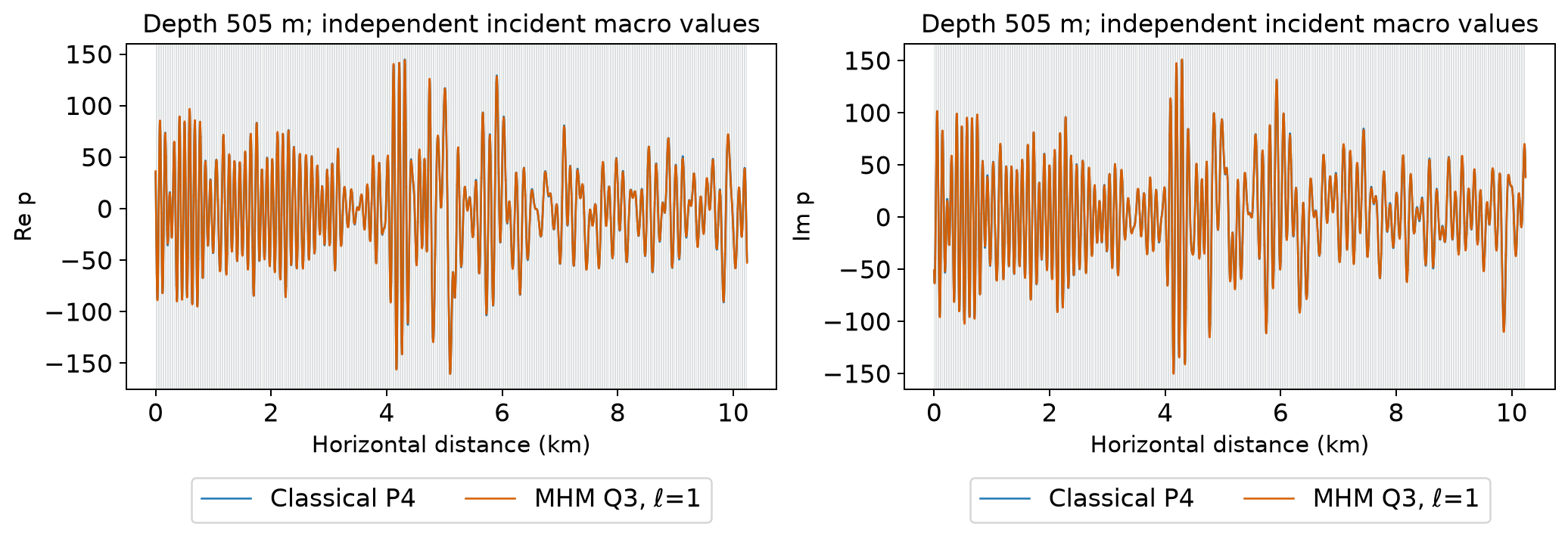
The unweighted \(513\times129\) sample norm is sensitive to the incident macro selected at an interface. Here the signs select the incident side in horizontal and depth coordinates, respectively:
| Incident side | Sampled pressure difference |
|---|---|
| \((-1,-1)\) | 2.77705% |
| \((-1,+1)\) | 2.68221% |
| \((+1,-1)\) | 2.94883% |
| \((+1,+1)\) | 2.79895% |
The published Table 6.1 value, 2.90%, falls inside this interval. Numerical proximity does not identify the article's material arrays or its incident sampling convention. All four incident-side conventions use the same pinned crop, unit source and declared approximation spaces. The MHM acquisition and physical comparison retain the exact archive digests and all four sample conventions.
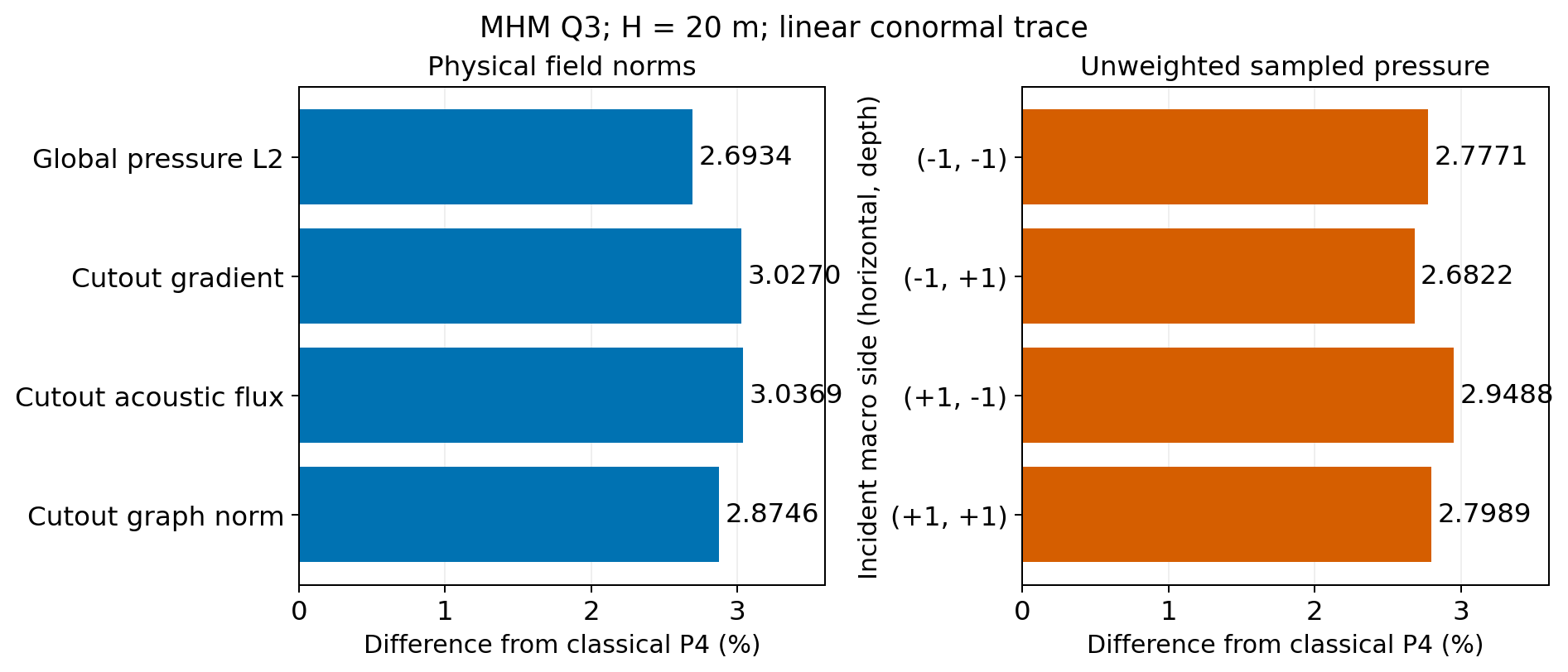
Physical integration and unweighted vertex sampling are shown separately. The four sampling bars preserve the original incident-side values without averaging them.
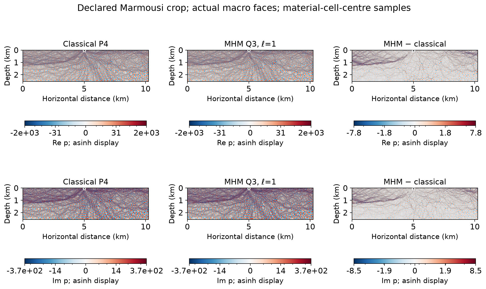
These maps sample the centres of the original material cells. Their common pressure scales include the complete native nodal extrema; the difference scale includes all plotted differences. The one-sided profiles below use independent values at each intersected macroface, at depth 505 m, away from the point source.
Classical complex fields and profiles
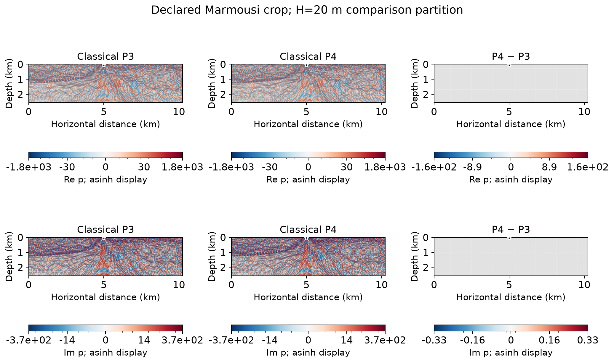
The pressure panels compare classical \(P_3\) and \(P_4\) fields on the same pixel-conforming material mesh. The \(H=20\) m overlay identifies the MHM comparison partition; it does not change either classical space. The star marks the point source.
The signed real and imaginary maps retain every native nodal value, including the source node. Color limits include the full nodal ranges, with a shared scale for the two references in each row. The difference is evaluated on the \(P_4\) nodal grid. The displayed asinh transform has linear width 1; colorbar ticks give original field values. It changes the display only, without clipping or normalizing the pressure coefficients.
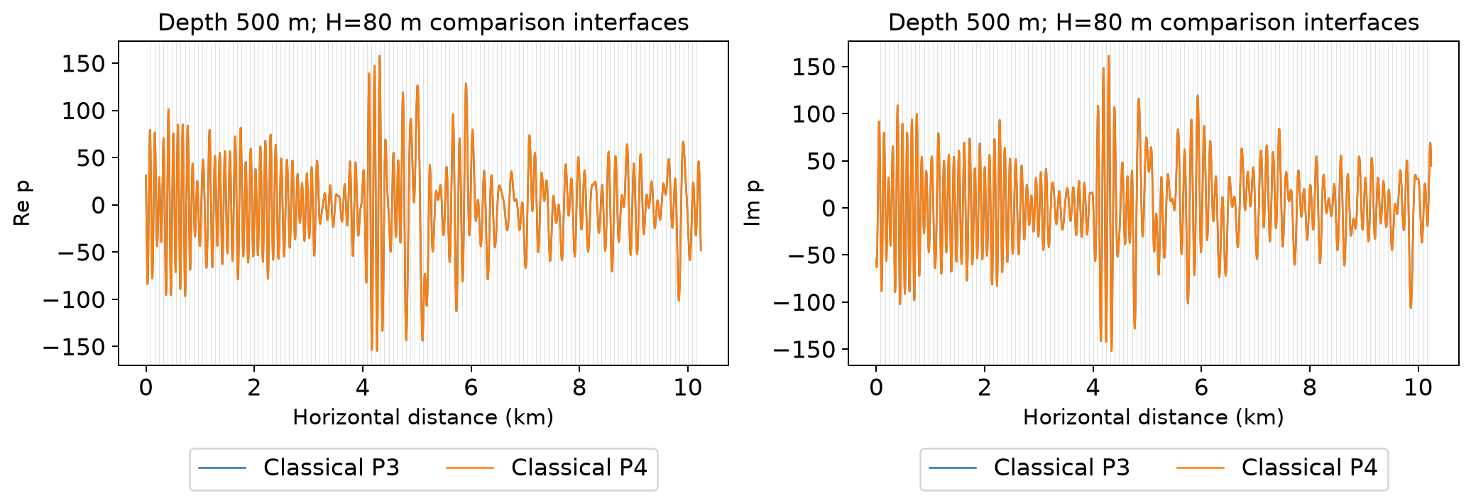
Profiles at depth 500 m avoid the source and use linear amplitude axes. Vertical markers show the \(H=80\) m comparison-face intersections.
The field-display record identifies the complete \(Q_3\), \(P_3\) and \(P_4\) arrays, material digests and observed native runtime used by these field maps and profiles. The norm tables and summary plots retain their original acquisition records and square-cutout convention; the spatial figures show pressure over the entire declared crop.
Execution
The importable examples.marmousi_data.download_marmousi_data helper acquires
the two primary SEG-Y files at the stated URLs. It checks exact file size and
SHA-256, reuses verified cached files and exposes each completed download
atomically. The numerical loader continues to require verified local files.
The following locked commands acquire and inspect the classical \(P_1\) level:
pixi run --locked -e notebooks python -m examples.marmousi_data --directory build/data/marmousi
pixi run --locked -e fem mpiexec -n 4 python -m examples.marmousi_reference \
  --data build/data/marmousi --degree 1
pixi run --locked -e notebooks python -m examples.marmousi_fields \
  examples/results/marmousi/classical-p1.json --data build/data/marmousi
The MHM driver exposes the published macro/local configuration explicitly:
pixi run --locked -e notebooks python -m examples.marmousi_campaign \
  --data build/data/marmousi --H 20 --trace-degree 1 --workers 8
This complete MHM configuration has tens of millions of local complex coefficients and dense local response maps. The trace-family driver can store these responses in independently verified batches and release them before the global factorization. Reconstruction reads the original response coefficients without changing precision, quadrature or the discrete operator.
pixi run --locked -e notebooks notebooks-run 72 executes the current full-crop
physical problem with Q1 local fields and P0 conormal traces on a 32×8 macrogrid.
It acquires both pinned primary datasets automatically, solves through the
public local/global equations and compares two exact-pixel quadrature orders
and the independently assembled original block system. This coarse
configuration checks the current operator; its physical approximation accuracy
is not established by a small residual or quadrature difference. The pinned
data occupy approximately 310 MB and the measured two-order control takes about
three minutes on the acquisition machine.
pixi run --locked -e notebooks notebooks-run 72 --study --plan lists the complete
current scientific acquisition: classical \(P_1\) through \(P_4\) references, the
stated \(H=20\) MHM configuration, norm comparisons and physical figures. Omitting
--plan executes those complete producer stages. They use the same complete
crop and point-source problem; their native factorizations require substantial
RAM, disk and execution time. The archive budget can be specified with
--max-data-bytes.
Field records include material provenance, executed-source hashes,
archive digests and original-equation residuals.
For a fixed macro width, the five polynomial conormal spaces are nested. The trace-family driver prepares degree four once and uses the exact coefficient injection \(T_\ell\) to solve
Here the real and imaginary coordinates remain interleaved. The original local matrices, source responses and trace lifts are shared; the absorbing boundary functional and the prescribed trace coordinates use the same restriction. All five degrees use volume and boundary quadrature order nine. Structural zero entries in the stored boundary couplings are omitted without changing their action. Reconstruction checks the original local equations, and the global residual tests the stated degree-\(\ell\) trace equations.
The trace-family verification compares restricted and direct solutions for all five degrees on small physical Marmousi patches at each of the three macro widths. The largest relative pressure difference is \(6.63\times10^{-14}\) and the largest relative trace difference is \(4.83\times10^{-14}\). These checks establish equivalence of the reuse procedure, not equality with the article's historical inputs. The corresponding command is
pixi run --locked -e intel python -m examples.marmousi_trace_family \
  --data build/data/marmousi --H 20 --workers 8 --solver pypardiso \
  --response-store build/checkpoints/marmousi-H20 --response-batch-size 1024
Each checkpoint binds the physical configuration, executed source hashes and
response-array digests. Resumption requires the same contract and verifies
every committed batch before reusing it. An interrupted, uncommitted batch is
recomputed. The portable scipy solver is also supported; the Intel command
above selects the nonsymmetric real PARDISO factorization of the interleaved
complex equations. Omitting --response-store keeps the responses in memory.
The retained records regenerate the norm-summary figures without field archives or new solves:
The complete field maps and profiles additionally require the acquired MPI nodal arrays and local MHM coefficients named in their acquisition records. These large arrays are not included in the package or notebook companion. Reference records also require the observed DOLFINx runtime attribution accepted by the archive reader. Independent comparison infrastructure supplies that observation; its sources are not distributed with PyMHM. The field-display record publishes the executed project revision, package identities and native binary digests. With complete current acquisitions available, the original plotting owners render the maps without changing the discrete spaces:
pixi run --locked -e notebooks python -m examples.plot_marmousi \
  --data build/data/marmousi --degrees 3 4
pixi run --locked -e notebooks python -m examples.plot_marmousi_mhm \
  examples/results/marmousi/mhm-H20-ell1.json \
  examples/results/marmousi/classical-p4.json
Notebook 72 defines the acoustic problem through the public local and global equations; its complete study mode acquires the reference and MHM fields explicitly.
References
-
Théophile Chaumont-Frelet, and Frédéric Valentin (2020). A Multiscale Hybrid-Mixed Method for the Helmholtz Equation in Heterogeneous Domains. SIAM Journal on Numerical Analysis 58(2) 1029-1067. DOI: 10.1137/19M1255616.
-
Gary S. Martin, Robert Wiley, and Kurt J. Marfurt (2006). Marmousi2: An elastic upgrade for Marmousi. The Leading Edge 25(2) 156-166. DOI: 10.1190/1.2172306.