Stokes–Brinkman boundary layers: MHM and MHM-USFEM
This complete application notebook contains the problem data, local and global equations, implementation and recorded results. For the general workflow, start with the method tutorials.
The main workflow is meshes → spaces → local equations → global balance → assemble → solve → fields and errors. MeshHierarchy associates macro and local meshes; bind_interface and LocalContext own supported numbering, geometric orientation and native coordinate conversions. The mathematical forms, physical trace meaning, local modes and gauge remain explicit in the cells below. Fully manual/custom spaces use the same numerical owners; see the custom-interface notebook.
We build the local mixed equations and the global skeletal equation explicitly. The classical baseline is an independently assembled, globally conforming Taylor–Hood P2/P1 solution on three fine meshes. We compare MHM with Taylor–Hood locals against MHM-USFEM with stabilized P2/P2 locals. Both MHM configurations use the same local velocity mesh, velocity degree and macroface space. We also assess the published single-element USFEM degree family independently of that Taylor–Hood comparison.
The analytical problem is the boundary-layer example in Araya, Harder, Poza and Valentin (2017), §3.1.2; its 2016 author preprint gives the equations and exact fields. This notebook uses a declared SW–NE triangulation. We distinguish the paper's single-element local degree family from the locally refined Taylor–Hood/USFEM comparison and from a resolved subface control. Geometry, coefficient, source and boundary data are the same throughout.
Open the downloaded notebook with jupyter lab after installing pymhm[notebooks,visualization] and the compatible native DOLFINx/UFL backend. Every physical field, source, variational form, boundary condition, pressure gauge and measurement is defined in the cells below. PyMHM assembles the executed UFL forms, integrates oriented traces, condenses local equations and solves the global system.
The PyMHM distribution contains only the library. The first cell explicitly
downloads a checksum-verified companion archive and prepares the declared data
using its local Python helpers. You can inspect these support files in ROOT.
Complete studies and historical replay retain their existing opt-in flags.
from pathlib import Path
import os
import sys
from pymhm.io.workspace import workspace_from_archive

# Download verified support files; this operation does not execute them.
COMPANION_URL = "https://ipes-lncc.github.io/pymhm/downloads/4b921d8289bdf4527c20b34c7a2bf234b6cc7abf8db1dc6f9dd8a6ec428cd7e4/stokes_brinkman_boundary_layer-companion.zip"
COMPANION_SHA256 = "4b921d8289bdf4527c20b34c7a2bf234b6cc7abf8db1dc6f9dd8a6ec428cd7e4"
WORKSPACE = Path(
    os.environ.get("PYMHM_WORKSPACE", Path.cwd() / ".pymhm-companions" / COMPANION_SHA256)
)
ROOT = workspace_from_archive(COMPANION_URL, sha256=COMPANION_SHA256, directory=WORKSPACE)
os.environ["PYMHM_WORKSPACE"] = str(ROOT)
if str(ROOT) not in sys.path:
    sys.path.insert(0, str(ROOT))

# Explicitly prepare declared data with the downloaded Python helpers.
from scripts.notebook_reproduction import notebook_workspace

ROOT = notebook_workspace("introduction/stokes_brinkman_boundary_layer.ipynb", directory=ROOT)
root = ROOT
print("Workspace:", ROOT)

import os

import json
import numpy as np
from pymhm import TriangleMesh, FaceSpace, SkeletonSpace
from pymhm.core.equations import Equation, LocalEquations
from pymhm.core.multiscale import assemble
from pymhm.fem.scalar.operators import triangle_quadrature, boundary_data
from pymhm.fem.scalar.triangle import nodal_space, tabulate

REPORTS = ROOT / "build/introduction"
REPORTS.mkdir(parents=True, exist_ok=True)
np.set_printoptions(precision=6, suppress=True)

from dataclasses import dataclass
from typing import Any
from threadpoolctl import threadpool_limits

threadpool_limits(limits=1)

from pymhm import MeshHierarchy, LocalContext, bind_interface, bind_problem
from pymhm.backends.spaces import bind_space

from functools import partial
from examples.introduction.vector import (
    flow_error_norms,
    record_brinkman_case,
    brinkman_reference,
    execution_provenance,
    plot_brinkman_convergence,
    plot_brinkman_family_rates,
    plot_brinkman_family_fields,
    plot_brinkman_enriched_fields,
    plot_brinkman_profiles,
)

measure_case = partial(record_brinkman_case, reports=REPORTS, root=ROOT)
Workspace: ./build/docs-restructure/final-workspaces/provenance-final-stokes_brinkman_boundary_layer-1476ab596271
Runtime setup: an owned UFL compiler cache
The local volume, pressure-mean and face forms use a notebook-owned temporary compiler cache. Its directory controls kernel storage only: operators, quadrature, approximation spaces, pressure gauge and solver checks are unchanged. We allow 7200 seconds for compilation; this timeout does not change any numerical tolerance.
Keep this cache alive while running the study. The final cell releases it after assembly, reference solves, error checks and plots are complete. Before another solve, rerun the cache-setup cell. After an interruption, call BRINKMAN_JIT_CACHE.cleanup() or restart the kernel before rerunning the setup. The local/global assembly in this tutorial remains serial.
from tempfile import TemporaryDirectory

BRINKMAN_JIT_CACHE = TemporaryDirectory(prefix="pymhm-brinkman-jit-")
BRINKMAN_JIT_OPTIONS = {"cache_dir": Path(BRINKMAN_JIT_CACHE.name), "timeout": 7200}
1. State the operator and derive the source independently
On the unit square, prescribe velocity on the whole boundary and fix the volume mean of pressure:
The published example sets \(\nu=10^{-2}\) and \(\gamma=1\). Define
The two velocity components depend on the opposite coordinate, so divergence is exactly zero. Since \(g''(s)=e^{(s-1)/\nu}/[\nu^2(1-e^{-1/\nu})]\), the independent source is
The PDE coefficient is \(\nu\), whereas the exponential layer width is \(\nu\) too; this is a manufactured example, not a homogeneous-forcing layer of width \(\sqrt{\nu/\gamma}\). In particular, replacing \(-\nu\Delta\) by \(-\nu^2\Delta\) would define another PDE. The stable exponential expression avoids overflow.
@dataclass(frozen=True)
class BrinkmanLayer:
    """The unit-square exact fields of Araya et al. (2017), section 3.1.2.

    The operator is ``-nu*Delta u+gamma*u+grad(p)`` and not ``-nu**2*Delta u``.
    The exact exponential layer has width ``nu``. Velocity is prescribed on
    the whole exterior; pressure ``x-y`` has zero volume mean. This example
    uses vector-Laplacian pseudostress, not symmetric Cauchy stress.
    """

    viscosity: float = 1e-2
    drag: float = 1.0

    def __post_init__(self) -> None:
        """Require positive viscosity and positive constant resistance for this tutorial."""
        if not np.isfinite(self.viscosity) or self.viscosity <= 0:
            raise ValueError("viscosity must be finite and positive")
        if not np.isfinite(self.drag) or self.drag <= 0:
            raise ValueError(
                "this tutorial requires finite positive drag; zero drag needs a local kernel"
            )

    def layer(self, coordinate: np.ndarray) -> np.ndarray:
        """Evaluate ``(exp((s-1)/nu)-exp(-1/nu))/(1-exp(-1/nu))`` stably."""
        return (np.exp((coordinate - 1) / self.viscosity) - np.exp(-1 / self.viscosity)) / (
            -np.expm1(-1 / self.viscosity)
        )

    def layer_derivative(self, coordinate: np.ndarray, order: int) -> np.ndarray:
        """Differentiate the exponential once or twice in physical coordinates."""
        if order not in (1, 2):
            raise ValueError("layer derivative order must be one or two")
        return np.exp((coordinate - 1) / self.viscosity) / (
            self.viscosity**order * -np.expm1(-1 / self.viscosity)
        )

    def velocity(self, points: np.ndarray) -> np.ndarray:
        """Return exact velocity ``(y-g(y), x-g(x))``."""
        reversed_points = points[:, ::-1]
        return reversed_points - self.layer(reversed_points)

    def pressure(self, points: np.ndarray) -> np.ndarray:
        """Return the mean-zero exact pressure ``x-y``."""
        return points[:, 0] - points[:, 1]

    def gradient(self, points: np.ndarray) -> np.ndarray:
        """Return velocity Jacobians with axes ``(point, component, derivative)``."""
        result = np.zeros((len(points), 2, 2))
        result[:, 0, 1] = 1 - self.layer_derivative(points[:, 1], 1)
        result[:, 1, 0] = 1 - self.layer_derivative(points[:, 0], 1)
        return result

    def source(self, points: np.ndarray) -> np.ndarray:
        """Apply the declared operator analytically, including ``grad(p)=(1,-1)``."""
        return (
            self.viscosity * self.layer_derivative(points[:, ::-1], 2)
            + self.drag * self.velocity(points)
            + np.array([1.0, -1.0])
        )
NU, GAMMA = 1e-2, 1.0
truth = BrinkmanLayer(NU, GAMMA)
# The main family fixes P2 velocity, P1/P2 pressure and P0 multipliers.
LOCAL_SUBDIVISIONS = 4
LOCAL_QUADRATURE_DEGREE, ERROR_ORDER = 28, 20
INVERSE_M = 1 / 100
points = np.array([[0.21, 0.34], [0.72, 0.81], [0.97, 0.98]])
np.testing.assert_allclose(np.trace(truth.gradient(points), axis1=1, axis2=2), 0.0)
np.testing.assert_allclose(
    truth.source(points)
    - GAMMA * truth.velocity(points)
    - NU * truth.layer_derivative(points[:, ::-1], 2),
    np.tile([1.0, -1.0], (len(points), 1)),
    atol=1e-12,
)
# Assumption (M), 2D: this Taylor--Hood submesh has interior vertices.
probe_local_mesh = TriangleMesh.unit_square(1).submesh(0, LOCAL_SUBDIVISIONS)
boundary_vertices = np.unique(probe_local_mesh.faces[probe_local_mesh.boundary_faces])
local_interior_vertices = len(probe_local_mesh.points) - len(boundary_vertices)
assert local_interior_vertices > 0
print("Taylor-Hood local interior vertices:", local_interior_vertices)
The NumPy expressions above provide physical data and independent error evaluation. The same explicit analytical data are written below as UFL expressions so that both local equations and the independent classical assembly integrate the actual exponential source.
import basix.ufl
import dolfinx
import ufl


def brinkman_ufl_data(domain: Any) -> tuple[Any, Any, Any]:
    """Write the exact velocity, pressure and independently derived source as UFL data."""
    x = ufl.SpatialCoordinate(domain)
    denominator = -np.expm1(-1 / NU)

    def g(s: Any) -> Any:
        """Evaluate the analytical exponential layer in UFL coordinates."""
        return (ufl.exp((s - 1) / NU) - np.exp(-1 / NU)) / denominator

    uexact = ufl.as_vector((x[1] - g(x[1]), x[0] - g(x[0])))
    pexact = x[0] - x[1]
    f = (
        ufl.as_vector(
            (
                ufl.exp((x[1] - 1) / NU) / (NU * denominator),
                ufl.exp((x[0] - 1) / NU) / (NU * denominator),
            )
        )
        + GAMMA * uexact
        + ufl.as_vector((1.0, -1.0))
    )
    return uexact, pexact, f
2. Translate the mathematical mixed form directly into UFL
Use the vector Laplacian form and its pseudostress, not the symmetric-strain Stokes operator:
The pressure test is negated to obtain a symmetric saddle matrix. For USFEM, the strong residual contains \(+\nabla p\):
These are the symmetric-test version of Eqs. (41)–(42) of the article. With constant scalar drag, the 2017 minimum-eigenvalue and 2025 maximum-eigenvalue conventions coincide. Here \(h_T\) is the actual fine-triangle diameter.
The comparison pair is P2/P2 with an unsplit P0 trace. It satisfies the sufficient condition \(k-\ell\geq d\) of Araya et al. (2025), Theorem 4.1. Four local subdivisions provide interior vertices for the Taylor–Hood comparison, as required by Assumption (M) in Section 4.2. The single-element degree family is stated separately below. We declare the conservative inverse parameter \(m=1/100\), then verify
on the actual P2 right triangles. This is an operator bound, not a value inferred from convergence. The Taylor–Hood P2/P1 submesh has three interior vertices on each macrotriangle and satisfies the stated local-mesh hypothesis; neither configuration introduces artificial pressure regularization.
from pymhm.fem.inequalities import laplacian_inverse_bound

# The bound is an operation on polynomial derivatives, independent of the PDE.
# Basix supplies the actual degree-dependent values; PyMHM owns the eigenproblem.
inverse_parameters, inverse_controls = {}, []
probe = TriangleMesh.unit_square(1)
bary, weights = triangle_quadrature(8)
for degree in (2, 3, 4):
    _, _, _, gradient, hessian = tabulate(probe, degree, bary)
    h = probe.lengths[probe.cell_faces].max(axis=1)
    selected = laplacian_inverse_bound(gradient, hessian, weights, h)
    np.testing.assert_allclose(selected, selected[0], rtol=1e-12, atol=1e-15)
    inverse_parameters[degree] = float(selected[0])
    stiffness = np.einsum("q,tqia,tqja->tij", weights, gradient, gradient)
    laplacian = np.trace(hessian, axis1=-2, axis2=-1)
    residual_gram = np.einsum("q,tqi,tqj->tij", weights, laplacian, laplacian)
    margins = np.linalg.eigvalsh(
        selected[:, None, None] * h[:, None, None] ** 2 * residual_gram - stiffness
    )[:, -1]
    assert margins.max() < 1e-10 * max(1.0, np.abs(stiffness).max())
    inverse_controls.append(
        dict(degree=degree, m=float(selected[0]), maximum_signed_margin=float(margins.max()))
    )
# The comparison's declared conservative P2 parameter also obeys the bound.
_, _, _, gradient, hessian = tabulate(probe, 2, bary)
stiffness = np.einsum("q,tqia,tqja->tij", weights, gradient, gradient)
laplacian = np.trace(hessian, axis1=-2, axis2=-1)
residual_gram = np.einsum("q,tqi,tqj->tij", weights, laplacian, laplacian)
bound_margins = np.linalg.eigvalsh(INVERSE_M * h[:, None, None] ** 2 * residual_gram - stiffness)[
    :, -1
]
assert bound_margins.max() < 1e-10
inverse_controls
[{'degree': 2,
  'm': 0.01041666666666667,
  'maximum_signed_margin': -2.5817457052426708e-16},
 {'degree': 3,
  'm': 0.003353888994497344,
  'maximum_signed_margin': 1.1237351776666785e-15},
 {'degree': 4,
  'm': 0.0012193412641237176,
  'maximum_signed_margin': 2.5062771001053377e-15}]
def brinkman_forms(
    domain: Any,
    *,
    stabilized: bool,
    velocity_degree: int = 2,
    inverse_m: float = INVERSE_M,
    quadrature_degree: int = LOCAL_QUADRATURE_DEGREE,
) -> tuple[Any, Any, Any, Any]:
    """Declare the executed vector-Laplacian mixed form and its USFEM residual."""
    pressure_degree = velocity_degree if stabilized else velocity_degree - 1
    element = basix.ufl.mixed_element(
        [
            basix.ufl.element(
                "Lagrange",
                "triangle",
                velocity_degree,
                shape=(2,),
                lagrange_variant=basix.LagrangeVariant.equispaced,
            ),
            basix.ufl.element(
                "Lagrange",
                "triangle",
                pressure_degree,
                lagrange_variant=basix.LagrangeVariant.equispaced,
            ),
        ]
    )
    W = dolfinx.fem.functionspace(domain, element)
    u, p = ufl.TrialFunctions(W)
    v, q = ufl.TestFunctions(W)
    dx = ufl.Measure("dx", domain=domain, metadata={"quadrature_degree": quadrature_degree})
    _, _, f = brinkman_ufl_data(domain)
    a = (
        NU * ufl.inner(ufl.grad(u), ufl.grad(v))
        + GAMMA * ufl.inner(u, v)
        - p * ufl.div(v)
        - q * ufl.div(u)
    ) * dx
    L = ufl.inner(f, v) * dx
    if stabilized:
        R = -NU * ufl.div(ufl.grad(u)) + GAMMA * u + ufl.grad(p)
        Rtest = -NU * ufl.div(ufl.grad(v)) + GAMMA * v + ufl.grad(q)
        h = ufl.CellDiameter(domain)
        tau = h**2 / (ufl.max_value(GAMMA * h**2, 4 * NU / inverse_m) + 4 * NU / inverse_m)
        a -= tau * ufl.inner(R, Rtest) * dx
        L -= tau * ufl.inner(f, Rtest) * dx
    return W, a, L, q * dx
The native mesh and coefficient conversions come from the shared backend binding. The provider below writes the mixed velocity–pressure volume forms and both oriented interface pairings, and registers velocity and pressure fields. Exterior velocity data enter the global trace equation; the physical pressure gauge is imposed after assembly.
import basix


from pymhm.backends.spaces import create_native_mesh, coefficient_map
from pymhm.backends.forms import assemble_form, assemble_pairing


def mixed_nodal_blocks(
    W: Any,
    a: Any,
    L: Any,
    mean_form: Any,
    fine: TriangleMesh,
    pressure_degree: int,
    velocity_degree: int = 2,
) -> tuple[Any, np.ndarray, np.ndarray, int]:
    """Compile supplied vector/scalar forms in declared canonical nodal coordinates."""
    binding = bind_space(fine, W)
    order = np.r_[
        coefficient_map(binding, component=0),
        coefficient_map(binding, component=1),
    ]
    native_A = assemble_form(a, jit_options=BRINKMAN_JIT_OPTIONS)
    native_F = assemble_form(L, jit_options=BRINKMAN_JIT_OPTIONS)
    A, F = native_A[order][:, order], native_F[order]
    pressure_weights = assemble_form(mean_form, jit_options=BRINKMAN_JIT_OPTIONS)[order]
    return A, F, pressure_weights, len(nodal_space(fine, velocity_degree)[1])
3. State trace orientation, boundary data and the physical gauge
With the global normal \(n_F\), the multiplier is the negative physical pseudotraction in that normal direction:
trace_coupling multiplies that globally oriented basis by each incident macrocell's outward-normal sign and integrates it against velocity. Thus local equations are \(A_Kw_K+B_K\lambda=F_K\), where \(w_K\) stores coefficients of the mixed physical fields \((\boldsymbol u_K,p_K)\) in the executed local basis. Choosing \(C_K=-B_K^\mathsf T\) makes the global equation
The right-hand side is a velocity moment, not prescribed traction. All exterior velocity data are imposed weakly by this equation. Equation(0,-boundary) makes its sign explicit. Positive drag removes the velocity-translation kernel, so there are no retained kernel amplitudes here.
Whole-boundary velocity data leave a global pressure constant undetermined. mean_constraint lifts the explicit local pressure weights into a global row. We constrain the physical reconstructed pressure integral; pinning a skeletal coefficient would generally choose a different gauge.
The provider below binds the mixed velocity–pressure space to the local mesh, writes both UFL interface pairings independently, and registers named velocity and pressure fields. A shared native coefficient adapter supplies the executed mixed representation used by the following norms and archives. The pressure mean form remains explicit for the global physical gauge.
def local_brinkman(
    local: LocalContext,
    *,
    macro: TriangleMesh,
    skeleton: SkeletonSpace,
    stabilized: bool,
    subdivisions: int = LOCAL_SUBDIVISIONS,
    velocity_degree: int = 2,
    inverse_m: float = INVERSE_M,
    quadrature_degree: int = LOCAL_QUADRATURE_DEGREE,
) -> LocalEquations:
    """Connect the declared mixed UFL equations to their oriented skeletal coordinates."""
    fine = local.mesh
    pressure_degree = velocity_degree if stabilized else velocity_degree - 1
    W, a, L, mean_form = brinkman_forms(
        create_native_mesh(fine),
        stabilized=stabilized,
        velocity_degree=velocity_degree,
        inverse_m=inverse_m,
        quadrature_degree=quadrature_degree,
    )
    A, F, pweights, nv = mixed_nodal_blocks(
        W, a, L, mean_form, fine, pressure_degree, velocity_degree
    )
    binding = local.native_space(W)
    u, p = ufl.TrialFunctions(W)
    v, q = ufl.TestFunctions(W)
    pair_b = local.trace_pairings(lambda phi, ds: ufl.inner(phi, v) * ds)
    pair_c = local.trace_pairings(lambda phi, ds: -ufl.inner(phi, u) * ds, axis="rows")
    order = np.r_[coefficient_map(binding, component=0), coefficient_map(binding, component=1)]
    B = assemble_pairing(
        pair_b.forms, axis="columns", jit_options=BRINKMAN_JIT_OPTIONS
    )[order]
    C = assemble_pairing(
        pair_c.forms, axis="rows", jit_options=BRINKMAN_JIT_OPTIONS
    )[:, order]
    # Preserve the declared (canonical velocity, canonical pressure) record layout.
    identity = np.eye(len(F))
    native_layout = binding.to_native(identity[: 2 * nv], component=0) + binding.to_native(
        identity[2 * nv :], component=1
    )
    local.field("velocity", binding, component=0, reconstruction=native_layout)
    local.field("pressure", binding, component=1, reconstruction=native_layout)
    return local.equations(
        a=A,
        L=F,
        b=B,
        c=C,
        metadata={
            "mesh": fine,
            "velocity_nodes": nv,
            "velocity_degree": velocity_degree,
            "inverse_m": inverse_m if stabilized else None,
            "pressure_degree": pressure_degree,
            "pressure_weights": pweights,
        },
    )
Before the refinement loop, define the measurements: velocity and pressure \(L^2\) errors, velocity-gradient error, broken pseudostress error, the fine-cell divergence norm and the separate macro mass defect. These quadrature operations evaluate fields; they do not define a local PDE.
The measurements use the general Basix kernel with the declared nodal order and affine geometry. The adapter below requests values and the first derivatives required by the norms; it does not select or assemble an operator.
Physical norms, executed-state archives and one-sided field/profile displays are importable from examples/introduction/vector.py. The local forms and the complete global solve remain in this notebook, together with separately declared conforming reference forms.
Record the numerical coordinates for reproducibility
The next utility saves the actual local coordinate basis, coefficients, orientation maps and reconstructed fields as each solve finishes. It contains no physical operator. Replaying the saved basis is checked with one and two BLAS threads; this positive-reaction or positive-drag example has no local nullspace modes. You can read the global construction immediately below without studying the archive format first.
def solve_brinkman_case(
    n,
    stabilized,
    *,
    subdivisions=LOCAL_SUBDIVISIONS,
    degree=2,
    trace_degree=0,
    segments=1,
    inverse_m=INVERSE_M,
):
    """Declare the mesh, trace space, weak velocity data and physical pressure gauge."""
    macro = TriangleMesh.unit_square(n)
    skeleton = SkeletonSpace(
        macro, tuple(FaceSpace.uniform(trace_degree, segments) for _ in macro.faces), components=2
    )
    boundary, fixed = boundary_data(skeleton, truth.velocity, {}, order=32)
    assert not fixed  # All exterior velocity data enter the global trace load.
    provider = lambda local: local_brinkman(
        local,
        macro=macro,
        skeleton=skeleton,
        stabilized=stabilized,
        subdivisions=subdivisions,
        velocity_degree=degree,
        inverse_m=inverse_m,
    )
    hierarchy = MeshHierarchy(
        macro, tuple(macro.submesh(c, subdivisions) for c in range(len(macro.cells)))
    )
    problem = bind_problem(
        hierarchy,
        bind_interface(skeleton, convention="normal"),
        provider,
        global_equation=Equation(0, -boundary),
        retained=0,
    )
    system = assemble(problem)
    gauge = system.mean_constraint(
        [data["pressure_weights"] for data in system.local_metadata], 0.0
    )
    solution = system.solve(constraints=[gauge])
    return macro, skeleton, system, solution, gauge


METHODS = (("MHM Taylor-Hood", False), ("MHM-USFEM", True))
cases, rows, state_archives = {}, [], []
for n in (4, 8, 16):
    for method, stabilized in METHODS:
        macro, skeleton, system, solution, gauge = solve_brinkman_case(n, stabilized)
        case, row, archive = measure_case(
            macro,
            skeleton,
            system,
            solution,
            truth,
            velocity_degree=2,
            pressure_degree=2 if stabilized else 1,
            order=ERROR_ORDER,
            name=f"brinkman-n{n}-{method.lower().replace(' ', '-')}",
            named=True,
            gauge=gauge if n == 4 else None,
            method=method,
            n=n,
        )
        cases[n, method] = case
        rows.append(row)
        state_archives.append(archive)
        print(
            method,
            n,
            {key: row[key] for key in ("velocity_l2", "pressure_l2", "macro_mass_defect")},
        )
MHM Taylor-Hood 4 {'velocity_l2': 0.3929962937977377, 'pressure_l2': 0.11142492150892233, 'macro_mass_defect': 1.0345457129856683e-15}
MHM-USFEM 4 {'velocity_l2': 0.3929259176980058, 'pressure_l2': 0.11241240860432737, 'macro_mass_defect': 2.3566489471688046e-15}
MHM Taylor-Hood 8 {'velocity_l2': 0.21599126611390915, 'pressure_l2': 0.06433041001089805, 'macro_mass_defect': 1.3109630568608477e-15}
MHM-USFEM 8 {'velocity_l2': 0.21596941590579988, 'pressure_l2': 0.06471481794611718, 'macro_mass_defect': 1.242278849233891e-15}
MHM Taylor-Hood 16 {'velocity_l2': 0.13349651144453092, 'pressure_l2': 0.044876506706566135, 'macro_mass_defect': 1.3172243244069515e-15}
MHM-USFEM 16 {'velocity_l2': 0.13349067858857142, 'pressure_l2': 0.0449591402455254, 'macro_mass_defect': 1.6500422041080057e-15}
Assess the published single-element degree family
Araya et al. (2017), Section 3.1 and Figures 6–8 uses one local triangle per macrotriangle and the equal-order family
We select these spaces explicitly, keeping the same analytical problem and global pressure gauge. The velocity_degree argument changes the UFL element, its executed field representation and interface integration together. There are no fine local submeshes in this experiment. The mesh parameter is the actual macrotriangle diameter \(H=\sqrt2/n\).
The paper reports eventual rates \(\ell+2\) for velocity \(L^2\) and \(\ell+1\) for pressure \(L^2\) and broken velocity-gradient error, with loss of rates while the layer is unresolved. These are literature observations for this example; the measured slopes below determine which regime our resolutions reach. The inverse coefficient is computed from each executed polynomial space, without using the exact solution or fitted error. The historical numerical inverse constants and connectivity are not supplied by the article, so this is a comparison of its PDE and degree family rather than a literal reproduction of its plotted values.
The default introductory profile uses \(n=8,16,32\) for each of the three degrees. It measures the same PDE and published approximation family on three resolutions; these levels can remain preasymptotic, so they do not establish the eventual literature rates. The main Taylor–Hood/USFEM study at \(n=4,8,16\), all three refined classical references, and the enriched face/local-space control are unchanged.
Set PYMHM_FULL_STUDY=1 before execution to acquire the original full
qualification sequence: \(n=8,16,32,64,128\) for \(\ell=0\) and
\(n=8,16,32,64\) for \(\ell=1,2\). The selected profile and actual levels are recorded
in the numerical provenance; either profile computes its own fields and slopes.
# Set PYMHM_FULL_STUDY=1 to extend each family to its complete qualification grids.
FULL_STUDY = os.environ.get("PYMHM_FULL_STUDY", "0") == "1"
PUBLISHED_FULL_LEVELS = {0: (8, 16, 32, 64, 128), 1: (8, 16, 32, 64), 2: (8, 16, 32, 64)}
PUBLISHED_LEVELS = PUBLISHED_FULL_LEVELS if FULL_STUDY else {ell: (8, 16, 32) for ell in (0, 1, 2)}
STUDY_PROFILE = "full qualification" if FULL_STUDY else "introductory three-mesh refinement profile"
print("Single-element family profile:", STUDY_PROFILE, PUBLISHED_LEVELS)
published_cases, published_rows = {}, []
for ell, levels in PUBLISHED_LEVELS.items():
    degree = ell + 2
    for n in levels:
        macro, skeleton, system, solution, _ = solve_brinkman_case(
            n,
            True,
            subdivisions=1,
            degree=degree,
            trace_degree=ell,
            inverse_m=inverse_parameters[degree],
        )
        case, row, archive = measure_case(
            macro,
            skeleton,
            system,
            solution,
            truth,
            velocity_degree=degree,
            pressure_degree=degree,
            order=ERROR_ORDER,
            name=f"brinkman-single-ell{ell}-n{n}",
            method="MHM-USFEM single element",
            ell=ell,
            local_degree=degree,
            n=n,
            local_subdivisions=1,
            inverse_m=inverse_parameters[degree],
        )
        published_cases[ell, n] = case
        published_rows.append(row)
        state_archives.append(archive)
        print(
            "single-element USFEM",
            ell,
            degree,
            n,
            {key: row[key] for key in ("velocity_l2", "pressure_l2", "velocity_h1_seminorm")},
        )
Single-element family profile: introductory three-mesh refinement profile {0: (8, 16, 32), 1: (8, 16, 32), 2: (8, 16, 32)}
single-element USFEM 0 2 8 {'velocity_l2': 0.22784628836433193, 'pressure_l2': 0.07469651596792912, 'velocity_h1_seminorm': 8.296979333667744}
single-element USFEM 0 2 16 {'velocity_l2': 0.13684729724035957, 'pressure_l2': 0.05087995811645847, 'velocity_h1_seminorm': 6.994233652188203}
single-element USFEM 0 2 32 {'velocity_l2': 0.06427039477956957, 'pressure_l2': 0.03214003264757917, 'velocity_h1_seminorm': 5.418213098615565}
single-element USFEM 1 3 8 {'velocity_l2': 0.0600439083609486, 'pressure_l2': 0.03135005926922251, 'velocity_h1_seminorm': 4.615242249111755}
single-element USFEM 1 3 16 {'velocity_l2': 0.021989892750822727, 'pressure_l2': 0.016737578281073574, 'velocity_h1_seminorm': 2.619558930811687}
single-element USFEM 1 3 32 {'velocity_l2': 0.0055097437352279195, 'pressure_l2': 0.0069172685098203976, 'velocity_h1_seminorm': 1.1444781448074353}
single-element USFEM 2 4 8 {'velocity_l2': 0.02413511833943785, 'pressure_l2': 0.01455038568775532, 'velocity_h1_seminorm': 2.497680308189383}
single-element USFEM 2 4 16 {'velocity_l2': 0.005237527262253736, 'pressure_l2': 0.005781670625628373, 'velocity_h1_seminorm': 0.8887876488192209}
single-element USFEM 2 4 32 {'velocity_l2': 0.0006940151358108268, 'pressure_l2': 0.0014560134273614688, 'velocity_h1_seminorm': 0.21153178616086232}
assembly_quadrature_controls = []
probe_macro = TriangleMesh.unit_square(PUBLISHED_LEVELS[0][0])
for ell in (0, 1, 2):
    degree = ell + 2
    probe_skeleton = SkeletonSpace(
        probe_macro, tuple(FaceSpace.uniform(ell) for _ in probe_macro.faces), components=2
    )
    candidates = np.flatnonzero(
        np.any(np.isclose(probe_macro.points[probe_macro.cells, 0], 1.0), axis=1)
    )
    cell_index = int(candidates[0])  # A macrotriangle touching the actual layer x=1.
    hierarchy = MeshHierarchy(
        probe_macro, tuple(probe_macro.submesh(c, 1) for c in range(len(probe_macro.cells)))
    )
    probe_problem = bind_problem(
        hierarchy, bind_interface(probe_skeleton, convention="normal"), lambda local: None
    )
    operators = [
        local_brinkman(
            probe_problem.local_context(cell_index),
            macro=probe_macro,
            skeleton=probe_skeleton,
            stabilized=True,
            subdivisions=1,
            velocity_degree=degree,
            inverse_m=inverse_parameters[degree],
            quadrature_degree=q,
        )
        for q in (LOCAL_QUADRATURE_DEGREE, max(40, LOCAL_QUADRATURE_DEGREE + 12))
    ]
    standard, higher = operators
    np.testing.assert_allclose(standard.a.toarray(), higher.a.toarray(), rtol=1e-11, atol=1e-13)
    np.testing.assert_allclose(standard.L, higher.L, rtol=1e-10, atol=1e-13)
    assembly_quadrature_controls.append(
        dict(
            ell=ell,
            local_degree=degree,
            cell=cell_index,
            quadrature_degrees=[LOCAL_QUADRATURE_DEGREE, max(40, LOCAL_QUADRATURE_DEGREE + 12)],
            matrix_maximum_difference=float(np.max(np.abs((standard.a - higher.a).toarray()))),
            load_maximum_difference=float(np.max(np.abs(standard.L - higher.L))),
        )
    )
assembly_quadrature_controls
[{'ell': 0,
  'local_degree': 2,
  'cell': 14,
  'quadrature_degrees': [28, 40],
  'matrix_maximum_difference': 1.9081958235744878e-16,
  'load_maximum_difference': 1.1102230246251565e-16},
 {'ell': 1,
  'local_degree': 3,
  'cell': 14,
  'quadrature_degrees': [28, 40],
  'matrix_maximum_difference': 3.7470027081099033e-16,
  'load_maximum_difference': 5.551115123125783e-17},
 {'ell': 2,
  'local_degree': 4,
  'cell': 14,
  'quadrature_degrees': [28, 40],
  'matrix_maximum_difference': 4.0245584642661925e-16,
  'load_maximum_difference': 1.1015494072452725e-16}]
Resolve the layer while retaining a simple macro mesh
The unsplit P0 sequence and the degree family assess their measured layer regime separately. A small algebraic residual and macro mass defect do not imply a resolved velocity gradient. To separate this limitation from the local mixed solver, we add a distinct resolution control: eight local subdivisions per macro edge and eight independent P0 subfaces per original macroface, on macro grids \(n=4,8,16\). The actual mesh scales are \(\mathcal H=\sqrt{2}/n\) for macrotriangles and \(\bar H=h=\mathcal H/8\) for their aligned subface and local partitions.
Both mixed methods retain P2 velocity and the same refined local mesh; pressure is P1 for Taylor–Hood and P2 for USFEM. Trace integration resolves the declared subfaces and includes the same orientation convention. This enriched skeletal discretization is reported separately from the unsplit polynomial experiment. We assess its physical errors, pressure gauge and macro balance through the same assembly; we do not transfer the paper's unsplit-face convergence theorem to this control.
At \(n=16\), the global geometry has only 512 macrotriangles, versus 32768 triangles in the classical reference. Fine resolution is confined to independent local problems and subface coefficients. Increasing only local resolution while leaving the trace fixed would retain the original face approximation error.
The initial enriched mesh remains relatively coarse compared with the layer width. Three mesh resolutions provide two observed slopes without assuming that the first pair is asymptotic.
control_rows, enriched_cases = [], {}
TRACE_SUBFACES, CONTROL_LOCAL_SUBDIVISIONS = 8, 8
for n in (4, 8, 16):
    for method, stabilized in METHODS:
        macro, skeleton, system, solution, _ = solve_brinkman_case(
            n, stabilized, subdivisions=CONTROL_LOCAL_SUBDIVISIONS, segments=TRACE_SUBFACES
        )
        case, row, archive = measure_case(
            macro,
            skeleton,
            system,
            solution,
            truth,
            velocity_degree=2,
            pressure_degree=2 if stabilized else 1,
            order=ERROR_ORDER,
            name=f"brinkman-enriched-n{n}-{method.lower().replace(' ', '-')}",
            method=method,
            n=n,
            trace_subfaces=TRACE_SUBFACES,
            local_subdivisions=CONTROL_LOCAL_SUBDIVISIONS,
        )
        enriched_cases[n, method] = case
        control_rows.append(row)
        state_archives.append(archive)
        print(
            "enriched",
            method,
            n,
            {key: row[key] for key in ("velocity_l2", "pressure_l2", "velocity_h1_seminorm")},
        )
enriched MHM Taylor-Hood 4 {'velocity_l2': 0.014890301506250278, 'pressure_l2': 0.007897821673562662, 'velocity_h1_seminorm': 2.5719509044515014}
enriched MHM-USFEM 4 {'velocity_l2': 0.01471621337101159, 'pressure_l2': 0.010804803489100819, 'velocity_h1_seminorm': 2.5585030756287943}
enriched MHM Taylor-Hood 8 {'velocity_l2': 0.0035786076339810093, 'pressure_l2': 0.0044223361037836195, 'velocity_h1_seminorm': 1.044425232660424}
enriched MHM-USFEM 8 {'velocity_l2': 0.003521612401268686, 'pressure_l2': 0.005566186665395186, 'velocity_h1_seminorm': 1.0307332924301857}
enriched MHM Taylor-Hood 16 {'velocity_l2': 0.0007287227636964459, 'pressure_l2': 0.0019685893704412152, 'velocity_h1_seminorm': 0.3863699116916705}
enriched MHM-USFEM 16 {'velocity_l2': 0.0007188233882701563, 'pressure_l2': 0.0024270780275819134, 'velocity_h1_seminorm': 0.3784068165706137}
4. Independently assemble a classical Taylor–Hood baseline
The fine reference is one conforming P2/P1 mesh, with no skeleton, local condensation or residual stabilization. DOLFINx/UFL assembles the same operator with the independently derived source. Velocity is prescribed strongly on all boundary nodes; pressure has the same zero-volume-mean gauge. Strong and weak boundary enforcement give different discrete spaces, so identical coefficients are not expected.
The native pressure test \(q\) supplies the volume-moment row. The reference solve eliminates the fixed velocity coordinates and adds one exact mean constraint. It uses the package's checked linear solver without changing its tolerances. We measure true errors in three fine meshes because an exact solution is available; a fine numerical solution remains a numerical baseline.
def classical_brinkman_forms(space):
    """Declare the separate conforming P2/P1 energy, source and pressure moment."""
    u, p = ufl.TrialFunctions(space)
    v, q = ufl.TestFunctions(space)
    domain = space.ufl_domain()
    uexact, pexact, f = brinkman_ufl_data(domain)
    dx = ufl.Measure("dx", domain=domain, metadata={"quadrature_degree": 20})
    a = (
        NU * ufl.inner(ufl.grad(u), ufl.grad(v))
        + GAMMA * ufl.inner(u, v)
        - p * ufl.div(v)
        - q * ufl.div(u)
    ) * dx
    return a, ufl.inner(f, v) * dx, q * dx, uexact, pexact, dx


references, reference_rows = {}, []
for n in (32, 64, 128):
    case, row, archive = brinkman_reference(
        n, classical_brinkman_forms, truth, reports=REPORTS, root=ROOT
    )
    references[n] = case
    reference_rows.append(row)
    state_archives.append(archive)
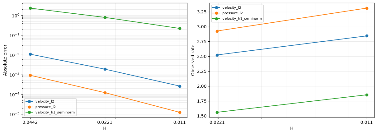
Conforming Taylor-Hood 32 {'velocity_l2': 0.010869696788162906, 'pressure_l2': 0.0009276145766838451, 'velocity_h1_seminorm': 2.3347183820122535, 'pressure_integral': -1.713039432527097e-17}
Conforming Taylor-Hood 64 {'velocity_l2': 0.0018898582823922592, 'pressure_l2': 0.00012204647106008795, 'velocity_h1_seminorm': 0.7917985117231211, 'pressure_integral': -1.543632843076237e-17}
Conforming Taylor-Hood 128 {'velocity_l2': 0.0002633185796566055, 'pressure_l2': 1.23030233163184e-05, 'velocity_h1_seminorm': 0.2190452313080452, 'pressure_integral': -8.2135090829355e-17}
5. Measure convergence, without assuming the asymptotic regime
\(H=\sqrt2/n\) denotes the actual maximum macrotriangle diameter. The Taylor–Hood/USFEM comparison has four local subdivisions per macro edge; the published degree-family experiment has one local triangle per macrotriangle. Their trace spaces and resulting measured errors are reported independently. The study keeps local degree, trace degree, subdivision factor, operator and boundary data fixed while halving \(H\).
A layer may be unresolved at the first levels. Plotting the observed rates makes this visible. The published smooth-space orders cannot be asserted before the exponential layer and the local approximation error are adequately resolved. The smallest singular value checks uniqueness of a particular gauged matrix; it does not establish a uniform inf-sup bound for an arbitrary mesh family.
The macro mass defect is \(\max_K\left|\int_K\nabla\cdot\boldsymbol u_h\right|\). It is distinct from the reported fine-cell divergence \(L^2\) norm: macro conservation does not make the raw velocity pointwise divergence-free.
For two successive resolutions, the measured slope is \(r=\log(e_1/e_2)/\log(H_1/H_2)\). These small plotting utilities compute that quantity directly and keep error and rate axes separate.
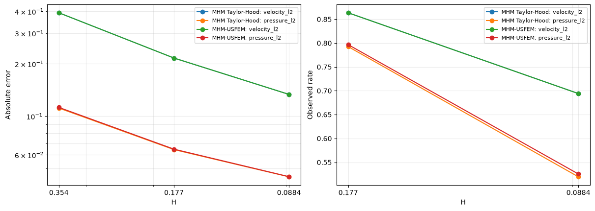
MHM Taylor-Hood: velocity_l2 rates: [0.863543 0.694171]
MHM Taylor-Hood: pressure_l2 rates: [0.792499 0.519541]
MHM-USFEM: velocity_l2 rates: [0.86343  0.694088]
MHM-USFEM: pressure_l2 rates: [0.796633 0.525482]
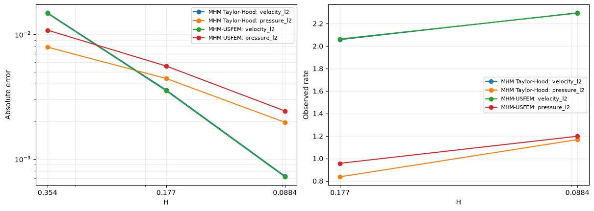
enriched MHM Taylor-Hood: velocity_l2 rates: [2.056903 2.295956]
enriched MHM Taylor-Hood: pressure_l2 rates: [0.836646 1.167646]
enriched MHM-USFEM: velocity_l2 rates: [2.063098 2.292527]
enriched MHM-USFEM: pressure_l2 rates: [0.956912 1.197469]
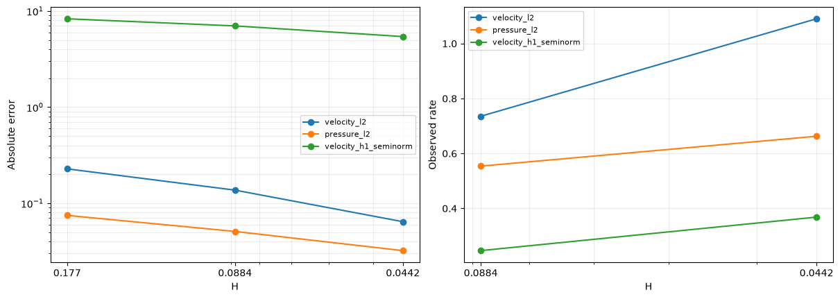
single-element 0 measured rates {'velocity_l2': [0.7354939276379141, 1.090340702249332], 'pressure_l2': [0.5539434706636922, 0.6627260885285837], 'velocity_h1_seminorm': [0.2464202005683821, 0.36834885616251173]}
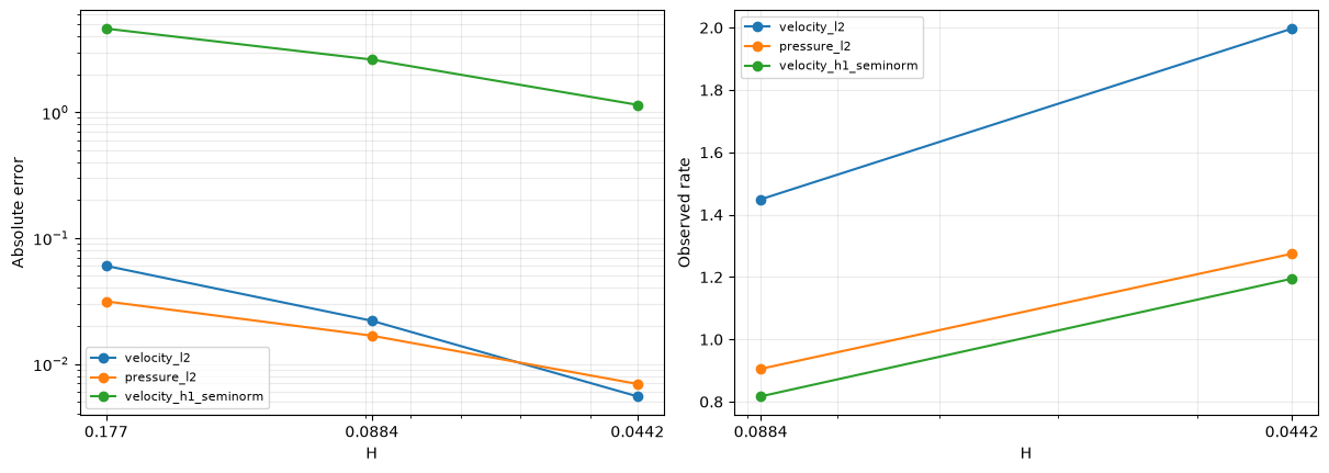
single-element 1 measured rates {'velocity_l2': [1.449177319615901, 1.9967834438956886], 'pressure_l2': [0.9053773675338614, 1.2748164388241332], 'velocity_h1_seminorm': [0.8170824574643614, 1.1946340047560302]}
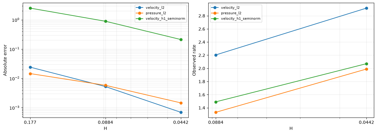
single-element 2 measured rates {'velocity_l2': [2.20417614720322, 2.915846816246214], 'pressure_l2': [1.3314990674458533, 1.9894627625297587], 'velocity_h1_seminorm': [1.4906781569715497, 2.0709642997184434]}
6. Inspect velocity, pressure, error and one-sided profiles
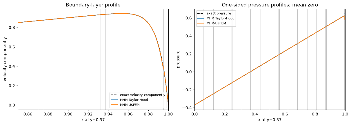
Every spatial panel highlights the actual macro mesh, including analytical and classical-reference panels. The fields are sampled from their original polynomials. Pressure remains independently reconstructed in each macrocell; coincident endpoints are not averaged. Velocity magnitude labels refer to velocity, not Darcy flux.
We show the enriched \(n=16\) MHM fields and a detailed profile in the layer near \(x=1\). The source has nonzero pressure gradient, so pressure accuracy is a separate measurement rather than a zero-pressure special case.
The display utility evaluates each local polynomial independently, including its one-sided boundary values. Every panel overlays the actual macro mesh and has its own color scale. It changes only the display sampling.
The additional single-element figure evaluates the \(\ell=2\), P4/P4 degree-family solution on its own macro mesh. Its coefficients and pressure mean come from that experiment, with no subface enrichment. The refined Taylor–Hood solution remains the independently assembled numerical baseline.
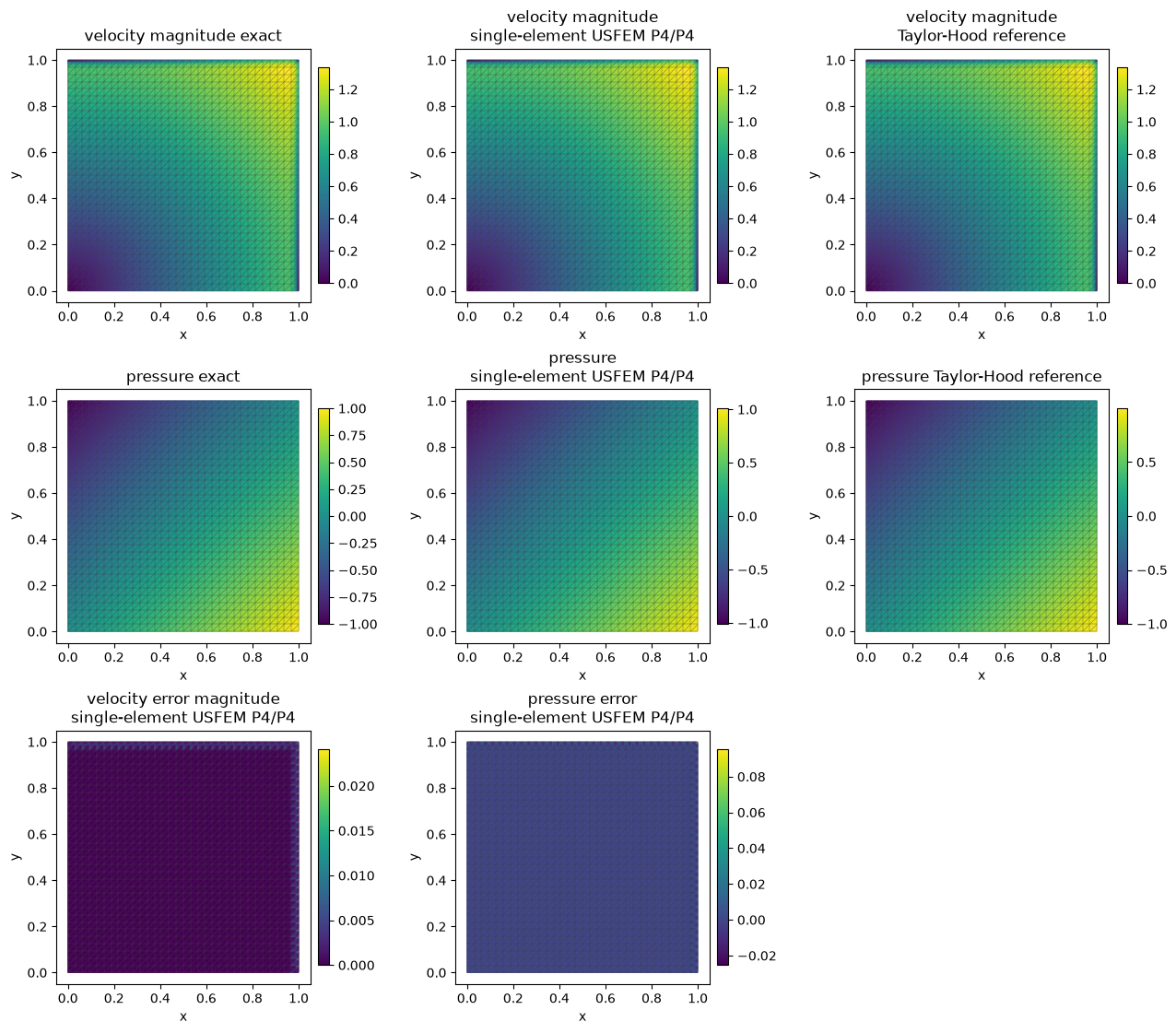
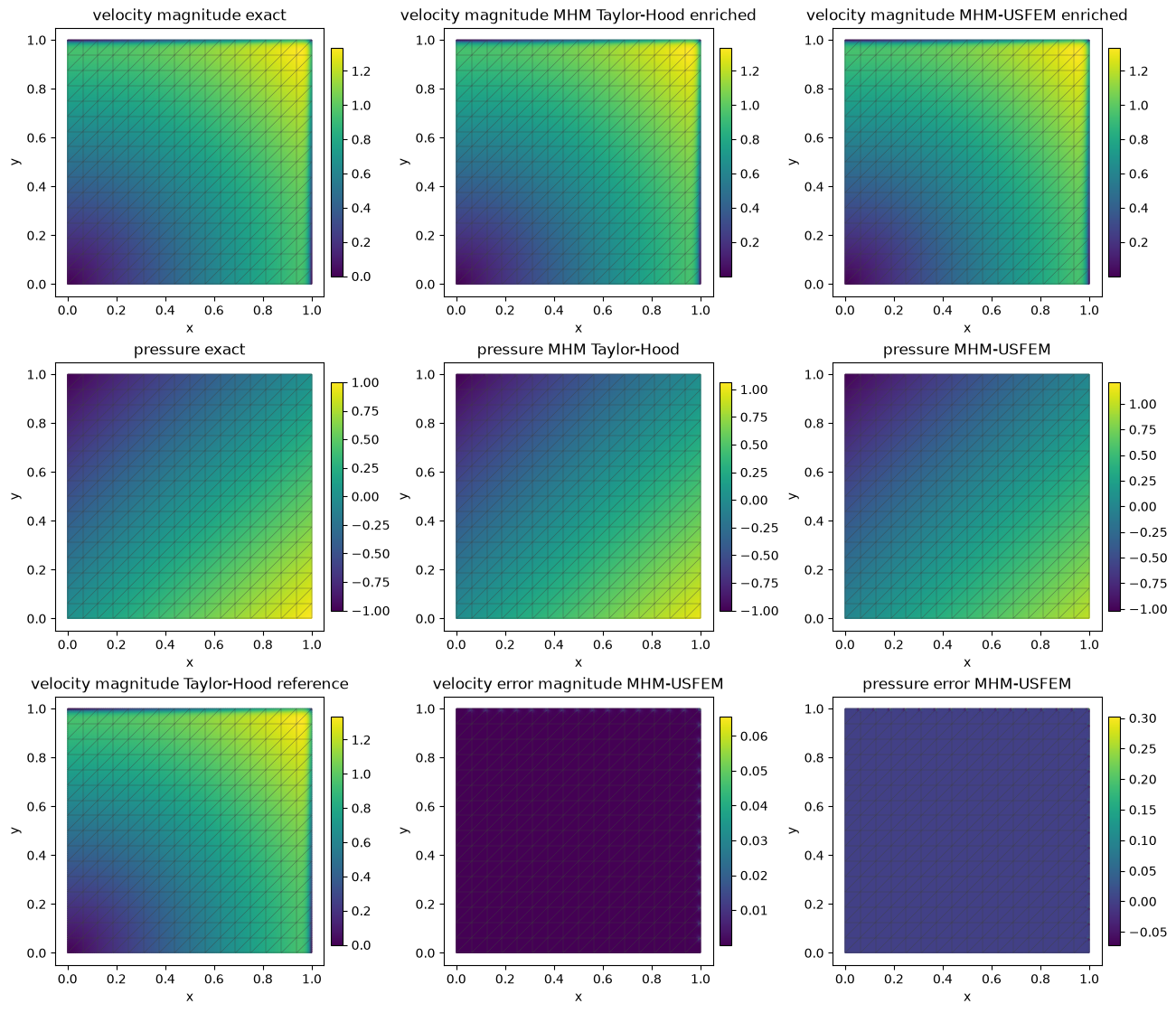
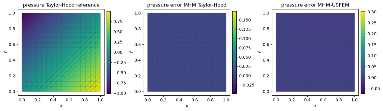
The classical pressure reference uses the same physical zero-mean gauge. The additional comparison below shows that field and the separate pressure errors of both multiscale methods.
Horizontal profiles retain a separate segment for each incident macrocell. Vertical markers identify macroface crossings; neighboring endpoint values are evaluated independently instead of being averaged.
7. Check quadrature and record the precise method provenance
Native local assembly uses UFL quadrature degree 28, and physical errors use 20 Gauss points in each Duffy coordinate. Reintegrating the finest MHM solution with 28 points checks that the layer norms are not quadrature artifacts. The baseline errors use a separately specified UFL degree-20 rule on the fine conforming meshes.
The raw pseudostress \(\nu\nabla\boldsymbol u_h-p_hI\) is a broken derived field. Its \(L^2\) error is reported, but we do not label it H(div) or infer fine-cell mass conservation. The singular-value and residual checks supplement the physical convergence and macro-balance measurements.
provenance = execution_provenance(
    "notebooks/introduction/stokes_brinkman_boundary_layer.ipynb",
    root=ROOT,
    native_jit_cache="notebook-owned temporary directory; removed after final result save",
    study_profile=STUDY_PROFILE,
    single_element_levels=PUBLISHED_LEVELS,
    full_qualification_levels=PUBLISHED_FULL_LEVELS,
    literature_comparison="same analytical PDE; declared tutorial discretization, no matched-figure reproduction",
)
quadrature_checks = {}
for method in ("MHM Taylor-Hood", "MHM-USFEM"):
    macro, meshes, u, p, pd = cases[16, method]
    higher = flow_error_norms(meshes, u, p, 2, pd, truth, order=28)
    measured = next(row for row in rows if row["n"] == 16 and row["method"] == method)
    for key in ("velocity_l2", "pressure_l2", "velocity_h1_seminorm", "pseudostress_l2"):
        np.testing.assert_allclose(higher[key], measured[key], rtol=1e-8, atol=1e-12)
    quadrature_checks[method] = higher
for method in ("MHM Taylor-Hood", "MHM-USFEM"):
    macro, meshes, u, p, pd = enriched_cases[16, method]
    higher = flow_error_norms(meshes, u, p, 2, pd, truth, order=28)
    measured = next(r for r in control_rows if r["n"] == 16 and r["method"] == method)
    for key in ("velocity_l2", "pressure_l2", "velocity_h1_seminorm", "pseudostress_l2"):
        np.testing.assert_allclose(higher[key], measured[key], rtol=1e-8, atol=1e-12)
    quadrature_checks[method + " enriched"] = higher
for ell in (0, 1, 2):
    selected = [row for row in published_rows if row["ell"] == ell]
    finest = selected[-1]
    macro, meshes, u, p, degree = published_cases[ell, finest["n"]]
    higher = flow_error_norms(meshes, u, p, degree, degree, truth, order=28)
    for key in ("velocity_l2", "pressure_l2", "velocity_h1_seminorm", "pseudostress_l2"):
        np.testing.assert_allclose(higher[key], finest[key], rtol=1e-8, atol=1e-12)
    quadrature_checks[f"USFEM single-element ell={ell}"] = higher
(REPORTS / "stokes-brinkman-boundary-layer.json").write_text(
    json.dumps(
        {
            "problem": "Araya et al. 2017 section 3.1.2, independently derived source",
            "source_url": "https://doi.org/10.1016/j.cma.2017.05.027",
            "viscosity": NU,
            "drag": GAMMA,
            "velocity_degree": 2,
            "local_subdivisions": LOCAL_SUBDIVISIONS,
            "pressure_degrees": {"MHM Taylor-Hood": 1, "MHM-USFEM": 2},
            "trace_degree": 0,
            "inverse_m": INVERSE_M,
            "inverse_bound_margin": float(bound_margins.max()),
            "boundary": "full velocity Dirichlet, weak MHM / strong conforming reference",
            "pressure_gauge": "zero physical volume mean",
            "reference_backend": f"DOLFINx {dolfinx.__version__}; independent P2/P1 UFL",
            "local_ufl_quadrature_degree": LOCAL_QUADRATURE_DEGREE,
            "error_duffy_order": ERROR_ORDER,
            "convergence": rows,
            "reference_refinement": reference_rows,
            "quadrature_checks": quadrature_checks,
            "enriched_control": control_rows,
            "single_element_family": published_rows,
            "single_element_rates": published_rates,
            "inverse_controls": inverse_controls,
            "assembly_quadrature_controls": assembly_quadrature_controls,
            "taylor_hood_local_interior_vertices": local_interior_vertices,
            "mesh_size_convention": "actual maximum macrotriangle diameter H=sqrt(2)/n",
            "theory_url": "https://doi.org/10.1137/24M1649368",
            "state_archives": state_archives,
            "provenance": provenance,
        },
        indent=2,
    )
)
The resulting rates describe these declared two-dimensional spaces and resolutions. The exact PDE and local residual are taken from Araya et al. (2017); the tutorial uses the explicitly declared SW–NE mesh and distinguishes the single-element P2/P2, P3/P3 and P4/P4 degree family from the refined P2 comparison. Reported pseudostress is a broken raw derived field. The independently assembled classical comparison uses DOLFINx through UFL and the project's checked sparse linear solver.
This configuration requires positive drag. In the pure Stokes limit, the vector-Laplacian local operator has two retained velocity translations in two dimensions; their basis moments and coarse amplitudes must be declared in the general problem API. That limit needs its own kernel configuration.
8. Compare the two smooth approximation families
The boundary-layer study above measures a difficult, distinct regime. To assess asymptotic approximation rates, use the smooth polynomial Stokes data with \(\nu=1\), \(\gamma=0\) and zero-volume-mean pressure:
These are the analytical data evaluated in the attributed PyMHM records. Section 3.1.1 of Araya et al. (2017) uses a negative streamfunction prefactor, so its velocity and force differ. This comparison assesses smooth convergence with the explicitly displayed data.
The same displayed volume form loses its reaction term. In this pure Stokes case, its two local null modes are \(Z_j=(e_j,0)\), \(j=1,2\). Particular local responses have zero velocity moments \(\int_T u_j\); their two translation amplitudes remain global unknowns (retained=2). The total physical velocity is not assigned zero mean. The pressure gauge remains the single physical condition \(\int_\Omega p=0\).
The two rate studies deliberately retain their different approximation spaces:
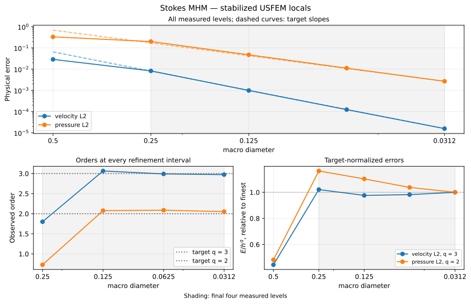
- MHM-USFEM: local stabilized P3/P3 on one triangle, P1 vector traces and a crisscross macro grid, \(H=1/n\).
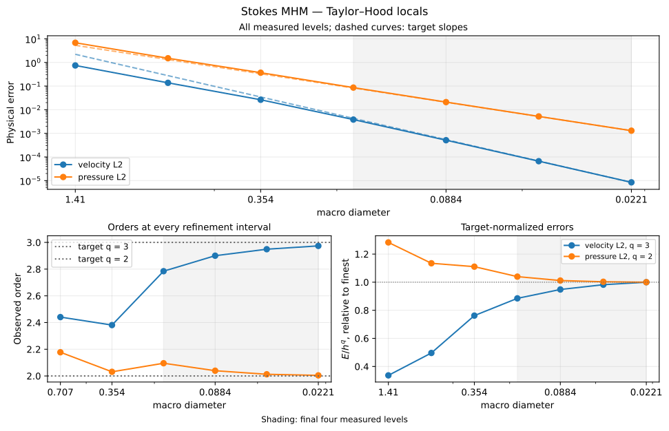
- MHM with Taylor–Hood locals: stable P2/P1 on 16 fine triangles per macrotriangle (four subdivisions per edge), P1 vector traces and the diagonal macro grid, \(H=\sqrt2/n\).
The Taylor–Hood local mesh satisfies the interior-vertex Assumption (M). Its P2/P1 locals and P1 trace have \(k-\ell=1\), outside the sufficient \(k-\ell\ge2\) condition of Araya et al. (2025), Theorem 4.3. The concrete saddle operator and trace lifting are checked independently; these finite checks do not extend that theorem. The USFEM P3/P3–P1 family meets Theorem 4.2, which estimates the broken velocity–pressure product norm rather than an additional velocity L2 order. Order-three velocity L2 and order-two pressure L2 are observed reference orders for these smooth studies. Araya et al. (2017), Section 2.2 states the general local stability and trace-lifting requirements.
Read the attributed acquisition records below. The graphs retain every measured level and show all consecutive orders; their highlighted window always uses the final four levels. Reading a numerical record does not recompute its PDE or change its recorded source identity. The independent local/global equation checks, pressure gauge and quadrature controls are recorded separately from the physical field errors.
import matplotlib.pyplot as plt
from IPython.display import SVG, display

from examples.tutorial_convergence import refinement_series, plot_method_series, asymptotic_summary

usfem_path = ROOT / "examples/results/stokes-adaptive/polynomial-uniform-nu1-g0-l1.json"
usfem_record = json.loads(usfem_path.read_text())
usfem_rows = [dict(row, H=2 / np.sqrt(row["macro_cells"])) for row in usfem_record["rows"]]
usfem_series = refinement_series(
    usfem_path, usfem_rows, "H",
    {"velocity L2": "velocity_l2", "pressure L2": "pressure_l2"},
    {"velocity L2": 3.0, "pressure L2": 2.0}, method="stokes-brinkman",
    spaces="Stabilized P3/P3 on one triangle; P1 vector traces; crisscross macro mesh",
    rate_provenance="Araya et al. (2017): observed velocity L2 order; Araya et al. (2025), Theorem 4.2: product-norm bound",
    refinement="macro diameter", root=ROOT,
)

hood_path = ROOT / "examples/results/tutorial-methods/stokes-taylor-hood-asymptotic.json"
hood_record = json.loads(hood_path.read_text())
hood_series = refinement_series(
    hood_path, hood_record["rows"], "H",
    {"velocity L2": "velocity_l2", "pressure L2": "pressure_l2"},
    {"velocity L2": 3.0, "pressure L2": 2.0}, method="stokes-galerkin",
    spaces="Taylor-Hood P2/P1, r4 local mesh; unsplit vector P1 traces; diagonal macro mesh",
    rate_provenance="Observed smooth refined Taylor-Hood family; k-ell=1 is outside the sufficient gap of Theorem 4.3 (2025)",
    refinement="macro diameter", root=ROOT,
)
for series in (usfem_series, hood_series):
    print(series["method"], "input", series["record"], "sha256", series["sha256"])
    print(asymptotic_summary(series))
    figure = plot_method_series(series)
    convergence_path = REPORTS / (series["method"] + "-smooth-convergence.svg")
    figure.savefig(convergence_path, bbox_inches="tight",
                   metadata={"Creator": "IPES Research Group", "Rights": "CC BY 4.0"})
    display(SVG(filename=str(convergence_path)))
    plt.close(figure)
stokes-brinkman input examples/results/stokes-adaptive/polynomial-uniform-nu1-g0-l1.json sha256 a2248fb906e8957977d57a746645b154acd63153edb0cc40ca7be46f354e8c68
{'velocity L2': {'start_index': 1, 'levels': 4, 'sizes': [0.25, 0.125, 0.0625, 0.03125], 'orders': [3.0644349493996885, 2.9913780094281828, 2.974092176861685], 'fitted_order': 3.0081093416496834, 'target': 3.0, 'amplitude_ratio': 1.0456753070099398}, 'pressure L2': {'start_index': 1, 'levels': 4, 'sizes': [0.25, 0.125, 0.0625, 0.03125], 'orders': [2.0771251271551012, 2.088109804627013, 2.0532112261882847], 'fitted_order': 2.07434482785382, 'target': 2.0, 'amplitude_ratio': 1.163479795696726}}
stokes-galerkin input examples/results/tutorial-methods/stokes-taylor-hood-asymptotic.json sha256 67678ccaa7fb23e2763b0ce10d36419a1b6f248bcbb1d205f8f6a66598fd9b21
{'velocity L2': {'start_index': 3, 'levels': 4, 'sizes': [0.1767766952966369, 0.08838834764831845, 0.04419417382415922, 0.02209708691207961], 'orders': [2.9005507938524766, 2.949144763672128, 2.974021185386308], 'fitted_order': 2.9420294992404856, 'target': 3.0, 'amplitude_ratio': 1.129969049618751}, 'pressure L2': {'start_index': 3, 'levels': 4, 'sizes': [0.1767766952966369, 0.08838834764831845, 0.04419417382415922, 0.02209708691207961], 'orders': [2.039192773068021, 2.012510326437911, 2.00432992832044], 'fitted_order': 2.0180609409917007, 'target': 2.0, 'amplitude_ratio': 1.0396032346901678}}
References
-
Rodolfo Araya, Christopher Harder, Abner H. Poza, and Frédéric Valentin (2017). Multiscale hybrid-mixed method for the Stokes and Brinkman equations—The method, Computer Methods in Applied Mechanics and Engineering 324, 29–53. DOI: 10.1016/j.cma.2017.05.027. Author preprint (2016): CI²MA Preprint 2016-15.
-
Rodolfo Araya, Christopher Harder, Abner H. Poza, and Frédéric Valentin (2025). Multiscale Hybrid-Mixed Methods for the Stokes and Brinkman Equations—A Priori Analysis, SIAM Journal on Numerical Analysis 63(2), 588–618. DOI: 10.1137/24M1649368.
Run this application notebook
View the source notebook or download the notebook, then open it:
python -m pip install 'pymhm[notebooks,visualization]'
jupyter lab stokes_brinkman_boundary_layer.ipynb
The first cell explicitly downloads a SHA256-verified companion archive. Acquisition does not execute its code. The local support files are inspectable in the printed ROOT directory; the following helper call prepares only the declared inputs. The library distribution contains only pymhm. Notebooks, support code and data are separate downloads. Native UFL forms require the compatible DOLFINx/UFL backend described in the installation guide. A clone and Pixi are unnecessary.
For batch execution, extract the same companion, change to its workspace, and use its local runner with the actual downloaded notebook path:
The runner uses the active Python interpreter and writes an executed copy and receipt under build/notebooks/introduction/. Larger data and field archives have documented download links and verified checksums.
The displayed figures and numerical outputs correspond to the retained validated execution of notebook SHA256 5c3b1a00d3651cea8bf2b41156b6a2a778ad6891078537dfb6f2c6c7b35ab472 in the publication manifest. Current instructions use the separately downloaded local examples and scripts support modules. Running the current source produces a separate receipt for its actual notebook, support bytes and environment. Timings describe the recorded hardware and solver settings; measure your own environment on an idle machine.