General tetrahedral degree and admissible P5/P2 estimation
The tetrahedral scalar adapter uses Basix Lagrange tabulation for positive polynomial degrees. Its nodes are the equispaced barycentric lattice, ordered by vertices, edges, faces and cell interior. PyMHM maps the Basix basis to this declared coefficient order and transforms derivatives through the affine tetrahedron map. The value/gradient-only path does not allocate Hessians. The conditioning of high-degree equispaced interpolation remains relevant; general-degree basis support is distinct from a formulation's degree and compatibility conditions.
Independent operator checks
P5 and P6 adapter checks match the physical nodes and derivative maps to Basix tabulation; this validates the adapter's conventions, not an independent implementation of the polynomial basis. Independent DOLFINx/UFL forms check the anisotropic stiffness, nonconstant source and every degree-two face coupling on a sheared tetrahedron. Additional tests cover cardinality, partition of unity, exact polynomial derivatives, positive mass, the single constant stiffness null mode, shared-node permutations and P8/P12 evaluation. Complete P5/P2 and P6/P2 quadratic Darcy patches include nonzero sources and inhomogeneous boundary data.
Assembly quadrature must resolve the selected polynomial products and data. The shared tetrahedral diffusion operator uses at least \(k+2\) Duffy points per coordinate. This exactness statement concerns polynomial products; nonpolynomial sources and error norms require separate checks.
Localized analytical problem
On the unit cube, use \(A=I\), homogeneous exterior pressure and
Analytical differentiation supplies the source and flux. Relative errors use the independently integrated volume norms \(\lVert p\rVert_{L^2}=0.121655888888664\) and \(\lVert q\rVert_{L^2}=1.25833145735624\). These are the same fields as the three-dimensional reconstruction study.
The sufficient degree condition for the estimator of Barrenechea et al. (2026) includes \(k\geq\ell+d\), \(\ell\leq m\leq k\), diffusion polynomial on each fine simplex and the theorem's regularity assumptions. The present local P5 / skeletal P2 configuration satisfies the three-dimensional boundary case \(5=2+3\). Both RT2 and RT3 reconstructions satisfy the stated range for \(m\). This is an original analytical verification, not a historical figure reproduction.
Five macro resolutions
The uniform sequence has \(6n^3\) macrotetrahedra for \(n=1,\ldots,5\), one fine tetrahedron per macrocell, and one P2 normal-flux polynomial per macroface. Coarse Gaussian integration uses assembly orders 34 and 18 for \(n=1,2\); subsequent levels use 12. Error checks use 34/38, 18/22 and 12/14, respectively. Every reported pressure, raw-flux and RT-flux norm is checked at both orders. The largest absolute change is below \(5.1\times10^{-10}\).
| Macrocells | Pressure L2 (%) | Raw flux L2 (%) | RT2 flux L2 (%) | Effectivity |
|---|---|---|---|---|
| 6 | 50.969092 | 74.664683 | 93.823207 | 9.70686 |
| 48 | 11.113485 | 26.410964 | 42.937140 | 8.70914 |
| 162 | 3.664716 | 11.044784 | 18.676529 | 7.33559 |
| 384 | 1.322437 | 5.514690 | 8.927786 | 5.57765 |
| 750 | 0.575218 | 3.001290 | 5.149386 | 5.67315 |
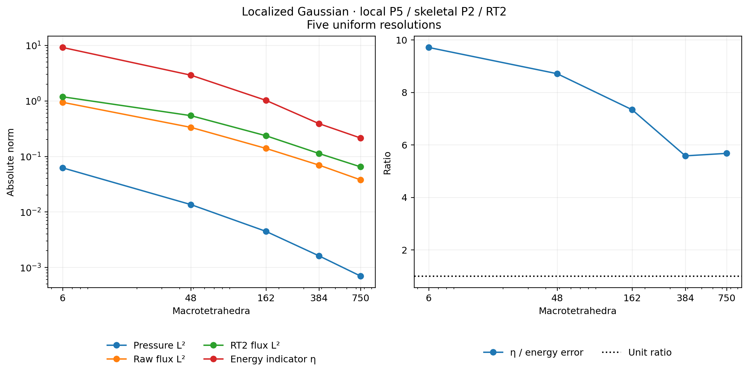
The errors decrease over all five recorded levels. The indicator-to-energy-error ratio remains greater than one in this sequence, but this finite set is not a proof of reliability for arbitrary meshes or data. The measured ratio includes flux defect, nonconformity, divergence defect and data oscillation.
Fixed geometry and reconstruction order
A separate control fixes 162 macrotetrahedra and 1,296 fine tetrahedra. Subdivision \(s=1\) assigns one P2 polynomial per original macroface; \(s=2\) assigns independent P2 polynomials to its four subtriangles. P4/P2 records are retained as physical-error comparisons only: they do not satisfy \(k\geq\ell+3\).
| Local degree | Subdivision | Reconstruction | Pressure L2 (%) | Raw flux L2 (%) | Reconstructed flux L2 (%) |
|---|---|---|---|---|---|
| 4 | 1 | RT2 | 2.046996 | 6.173829 | 6.936656 |
| 4 | 2 | RT2 | 0.159770 | 1.087139 | 3.242354 |
| 5 | 1 | RT2 | 2.040548 | 6.165486 | 6.888199 |
| 5 | 2 | RT2 | 0.124447 | 0.816917 | 2.936305 |
| 5 | 2 | RT3 | 0.124447 | 0.816917 | 1.472781 |
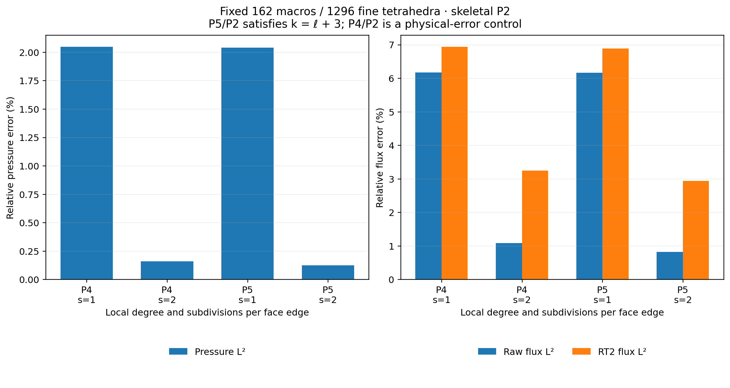
RT3 in the final row reconstructs the same P5 pressure and skeletal field as RT2; it does not solve another primal system. The canonical normal moments and continuous-test equilibrium residuals are below \(2.7\times10^{-15}\). The corresponding indicator ratios are 22.6545 for RT2 and 15.4024 for RT3. Canonical reconstruction is not an unconstrained L2 projection of the raw flux, so increasing its degree does not imply monotonic error reduction. Here the raw P5 gradient has degree four and is not generally contained in RT3.
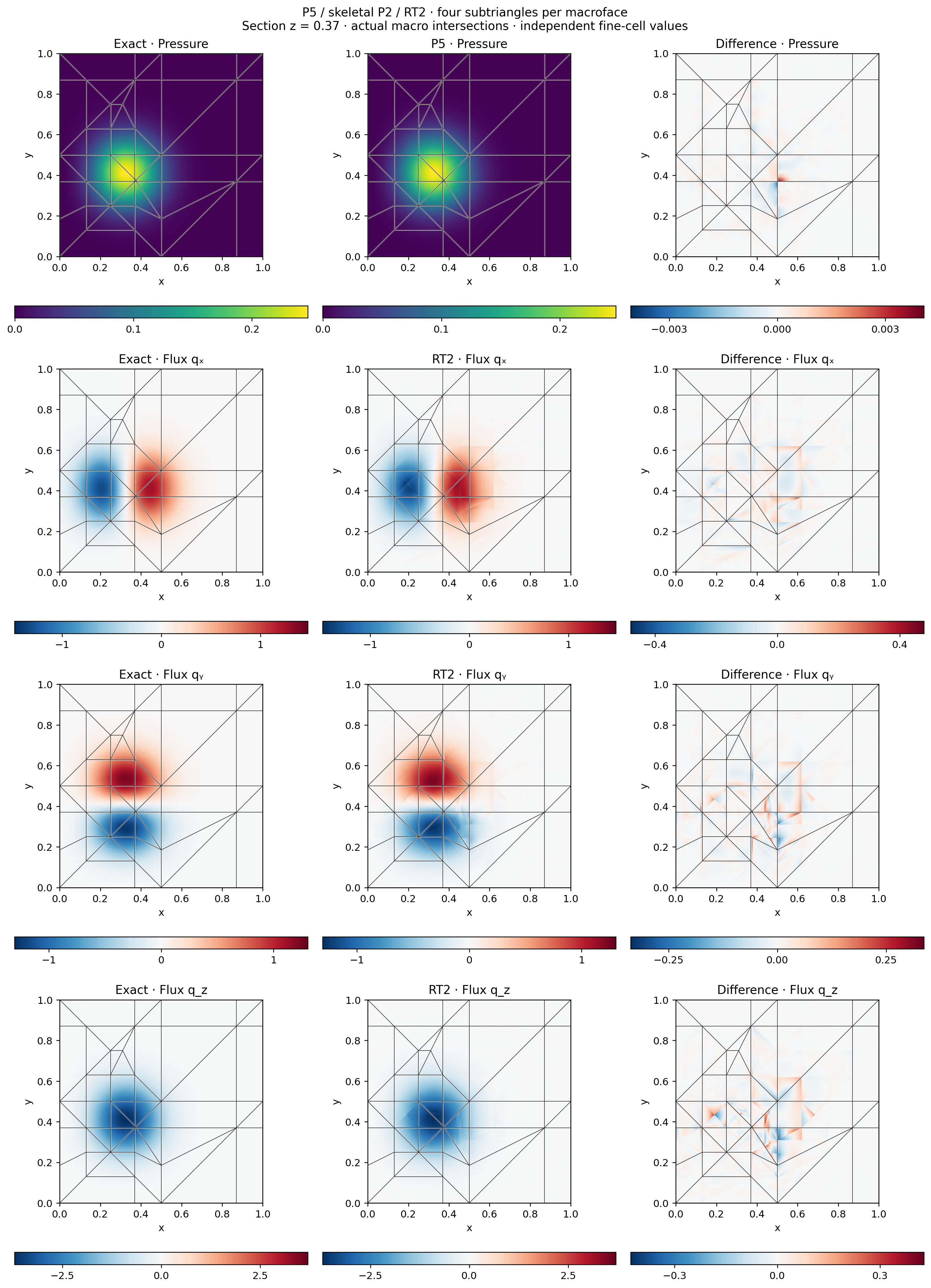
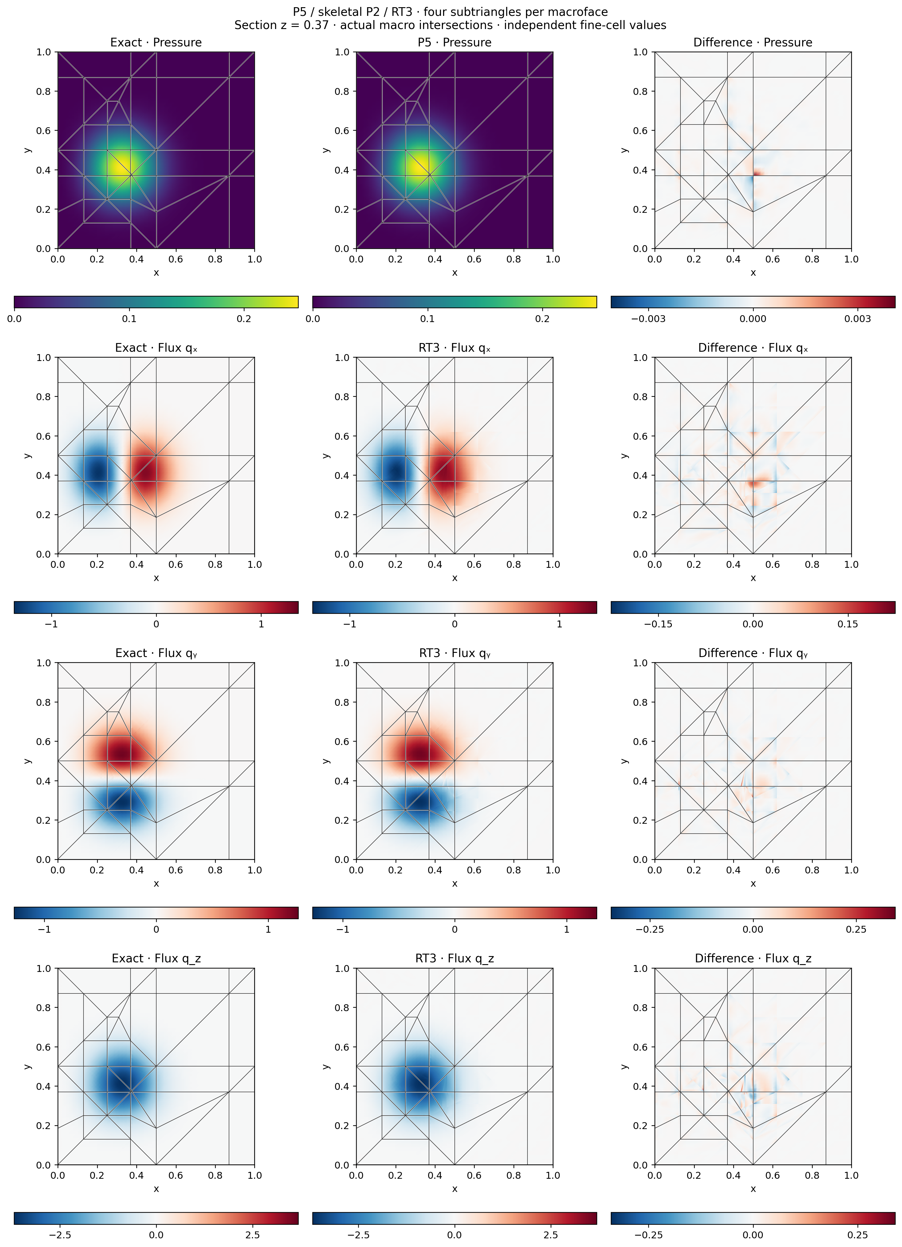
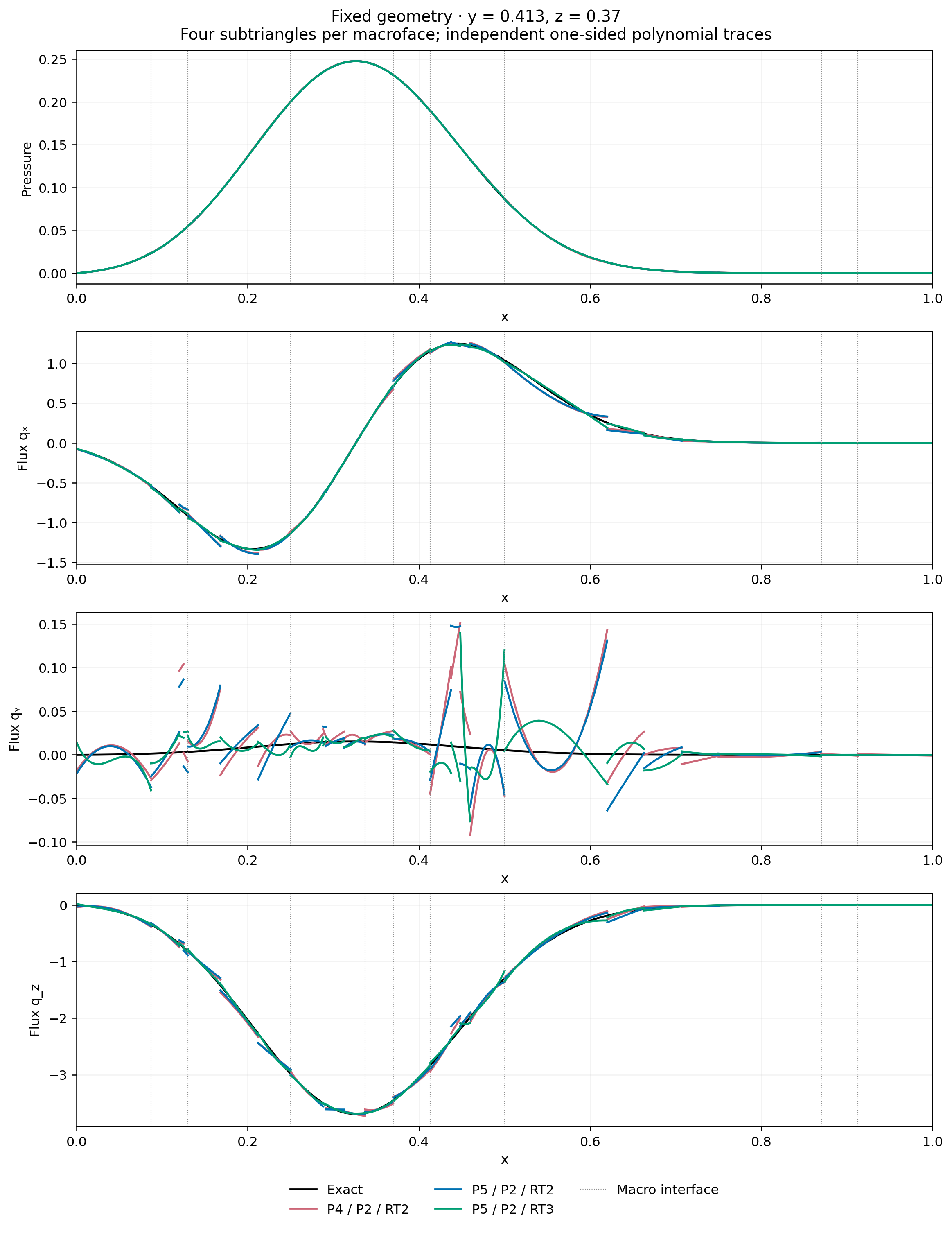
The field replay record identifies the original fixed-geometry discretization, executed RT bases and agreement of the acquired fields with the physical norms in the tables.
The slice is \(z=0.37\); profiles use \(y=0.413\). Every point is evaluated in its owning fine tetrahedron using the archived RT basis. Disconnected triangles and profile intervals preserve separate interface values. Exact and numerical component panels share limits, while signed differences have their own symmetric limits. Volume norms, rather than slice samples, quantify error. The chosen profile lies near the zero of the exact transverse component; its signed absolute deviations remain visible even when the combined vector norm is small. The continuous local moment conditions do not impose separate DG0 source balances on each fine tetrahedron; those residuals are recorded separately.
Reproduction
pixi run --locked -e test-core python -m examples.solve_tetra_pk uniform --workers 4
pixi run --locked -e test-core python -m examples.solve_tetra_pk fixed --workers 4
pixi run --locked -e test-core python -m examples.tetra_pk_reconstruction
pixi run --locked -e notebooks python -m examples.plot_tetra_pk
Records in examples/results/tetra-pk include quadrature checks, source and
archive digests, physical moments and the executed reconstruction basis.
Notebook 64 checks the archived data and displays the figures without rerunning
the numerical campaign. Run these commands from a repository checkout containing
the generated field archives. Release archives contain installation and build
sources; scientific examples, records and notebook resources remain in the
repository.
References
- Gabriel R. Barrenechea, Larissa Martins, Weslley Pereira, and Frédéric Valentin (2026). An H(div; Ω)-Conforming Flux Reconstruction for the Multiscale Hybrid-Mixed Method, Multiscale Modeling & Simulation 24(2), 399–428. DOI: 10.1137/24M1673073.