Darcy flux in SPE10 layer 36

The layer-36 Darcy experiment has a published flux-magnitude comparison in Barrenechea et al. (2026), §6.2, Figure 6. This complements the pressure maps and profiles of Paredes, Valentin and Versieux (2024), §5.2. The two articles use different approximation spaces. Their figures therefore provide distinct comparisons for the 66-square Darcy example.

Physical field and material convention

The calculation uses

\[ \Omega=(0,1200)\times(0,2200),\qquad q=-K\nabla p,\qquad \nabla\cdot q=0, \]

with \(p=1\) on the bottom, \(p=0\) on the top, and \(q\cdot n=0\) on the vertical sides. Both articles specify these boundary conditions for SPE10 Model 2, layer 36. The 2024 article explicitly sets the volume source to zero. The 2026 subsection does not separately restate its source value.

The distributed material is the horizontal tensor \(K=\operatorname{diag}(K_x,K_y)\) from the pinned OPM dataset. Layer numbers are one based. There are 60×220 material cells, each 20×10 ft; the arrays retain the original x/y orientation. On this layer, \(K_x=K_y\) exactly, with range 0.002163–8412.63 mD. Thus the in-plane tensor also equals \(K_x I\). The vertical component \(K_z\) and porosity do not enter this steady two-dimensional pressure equation.

The numerical fields retain permeability in mD, coordinates in ft, and the prescribed pressure values 1 and 0. The plotted flux is exactly \(-K\nabla p\) in this convention. Neither the pressure unit nor a viscosity conversion is specified in the article's flux experiment, so the published scale cannot be identified as an SI velocity scale. The 2026 subsection also does not state which tensor components were loaded. The component selection and units above describe the present calculation explicitly.

What Figure 6 publishes

Panel	Published field and discretization
Left	Magnitude of a standard mixed Raviart–Thomas order-2 reference flux; 125,000 triangles and 1,314,000 reported degrees of freedom
Middle	Magnitude of the raw flux \(-A\nabla u_{Hh}\), with local continuous P2 pressure and skeletal degree \(\ell=0\)
Right	Magnitude of the RT2 moment reconstruction from that MHM pressure, using \(m=2\)

All three colorbars have visible endpoints \(7.0\times10^{-9}\) and \(2.5\times10^{-2}\). Intermediate labels overlap in the original image. The paper does not specify the color transfer function, field-sampling locations, display interpolation, or whether the displayed endpoints are global extrema. These labels therefore do not define flux error norms. No vector-component maps, numerical flux profile, inlet flow rate, or field arrays accompany this figure in the inspected manuscript and repository record.

The MHM macroelement count and local refinement of Figure 6 are not stated explicitly. The subsequent adaptive experiment starts from 512 macroelements and four local elements per macroelement, and ends with 3,786 macroelements and 9,559 global unknowns. Those counts describe Figures 7–9; they cannot be assigned to Figure 6 without additional information. Figure 8 also shows flux magnitude, while Figure 9 shows a pressure profile along the diagonal from (0,0) to (1200,2200).

RT2 is distinct from BDM2

The article defines

\[ \mathrm{RT}_m(T)=[\mathbb P_m(T)]^2+x\mathbb P_m(T), \qquad \operatorname{div}\mathrm{RT}_m(T)=\mathbb P_m(T). \]

In two dimensions, RT2 has 15 local flux degrees of freedom: nine edge moments and six interior moments. BDM2 instead equals \([\mathbb P_2(T)]^2\), has 12 local degrees of freedom, and has divergence in P1. The BDM2/P1 Darcy solver consequently represents a different mixed pair from the published RT2 reference.

The paper does not identify whether its 1,314,000 count includes pressure. For illustration, a 250×250 rectangular grid split into 125,000 triangles has 188,000 edges, giving \(3(188000)+6(125000)=1314000\) RT2 flux coefficients. Adding independent P2 pressure would give 2,064,000 coefficients before boundary elimination. This arithmetic is consistent with a flux-only count; it does not establish the unpublished connectivity or pressure-space details of the reference.

Fixed MHM field and conforming Q3 comparison

The computed MHM field retains the 2024 face-based configuration:

Quantity	Configuration
Macrogrid	6×11 squares, each of side 200
Local pressure	Continuous Q1 on 120×120 quadrilaterals per macrocell
Skeleton	Continuous P1 on 32 segments of each macroface
Reduced global dimension	4,191 free trace coefficients plus 66 retained constants: 4,257
Material integration	Local cells aligned with the permeability pixels

Continuity of the skeletal basis is imposed within each macroface; values on different macrofaces are independent. The local refinement 120 is a declared choice because the 2024 article does not report that count. This quadrilateral Q1/continuous-P1 configuration is distinct from the triangular P2/P0 configuration in the flux-reconstruction figure.

The conforming comparison uses continuous Q3 pressure on a pixel-aligned 960×1760 quadrilateral grid: 1,689,600 elements and 15,214,561 coefficients. It solves the same declared material and boundary-value problem. This is a separate conforming assembly using PyMHM's basis and integration kernels, not an independent implementation or the article's mixed RT2 reference.

Flux magnitude describes conductive channels; signed components additionally resolve the direction of flow. A difference of magnitudes, \(\lvert q_{\mathrm{MHM}}\rvert-\lvert q_{\mathrm{Q3}}\rvert\), is not the vector difference \(q_{\mathrm{MHM}}-q_{\mathrm{Q3}}\). Likewise, a finite set of point samples does not define an integrated L2 norm. This report publishes the retained integrated comparisons and reference-refinement records. The original full coefficient and pixel-center field arrays needed to replay the Q3, MSL and NeoPZ spatial panels are not distributed with the checkout; scalar norms cannot be used to reconstruct those maps.

The MHM flux in these comparisons is the raw one-sided field \(-K\nabla p_h\). Its normal component can jump across fine and macro interfaces. Macro conservation instead follows from the skeletal flux: for every macrocell \(K\), the oriented integral of that flux equals \(\int_K f\). Small macro balance defects do not imply that the raw gradient field is H(div)-conforming or pointwise divergence-free.

The RT moment reconstruction is a separate algorithm on triangular submeshes. Its continuous-test-space conservation identity must not be strengthened to independent balance on every fine cell. Neither that reconstruction nor the published RT2 convergence estimate is implied by the raw quadrilateral Q1 flux comparison above.

Independent classical references

Two further comparisons use finite-element operators assembled by independent codes. Both retain the same layer, physical coordinates, coefficient pixels, source and boundary conditions. Their meshes fit the material pixels, and their approximation spaces differ from the MHM spaces and the article's RT2 reference.

Reference	Finest mesh	Unknowns before boundary elimination	Linear solver
PyMHM conforming Q3	960×1760 quadrilaterals	15,214,561	Intel MKL PARDISO through `pypardiso`
MSL_CG conforming P1	960×3520 rectangles split southwest–northeast; 6,758,400 triangles	3,383,681	Native MSL `LocalLinearSystem`, Eigen SparseLU
NeoPZ mixed RT0/P0	480×1760 rectangles split southwest–northeast; 1,689,600 triangles	4,226,240	Intel MKL PARDISO through `pypardiso`

The MSL execution uses msl_cg revision afb76d14c1baf50f0b9e69f7bcac675749ef4458 and msl_core revision 7f15f455717173d29080d411a7e732c72c1e87f8, with unchanged numerical libraries. It solves a global conforming P1 problem through DiffusionCGProblem; no MHM condensation is used in this reference. Pressure is prescribed strongly at the horizontal boundaries, and sidewall zero flux is natural. The reported physical field is its raw flux \(-K\nabla p_h\).

The NeoPZ revision uses TPZMixedDarcyFlow, triangular EHDivConstant order zero, and discontinuous constant pressure. Prescribed pressure enters the mixed boundary functional; sidewall normal-flux coefficients are eliminated exactly, without a penalty. Native NeoPZ supplies element assembly and physical-field evaluation. The sparse system is equilibrated and solved through pypardiso 0.4.7 with MKL 2026.1; its final residual is checked in the unscaled equations. This is the classical RT0/P0 method, not an execution of the NeoPZ MHM controller.

Integrated differences

For a reference field \((p_R,q_R)\), the relative differences are

\[ \begin{aligned} E_p&=\frac{\|p_{\mathrm{MHM}}-p_R\|_{L^2(\Omega)}} {\|p_R\|_{L^2(\Omega)}},\\ E_q&=\frac{\|q_{\mathrm{MHM}}-q_R\|_{L^2(\Omega)^2}} {\|q_R\|_{L^2(\Omega)^2}}. \end{aligned} \]

The flux norm integrates both vector components. It is not the difference of magnitudes or the RMS of the plotted pixel-center samples.

Reference for the fixed MHM field	Pressure difference, %	Vector-flux difference, %
Pixel-aligned Q3, 960×1760	0.208602	12.6093
MSL_CG P1, 960×3520	0.207577	12.6230
NeoPZ RT0/P0, 480×1760	0.257654	17.1396

For the Q3 comparison, integration uses the exact common rectangular partition of the two finite-element grids and the permeability pixels. On each intersection, pressure differences have coordinate degree at most three, and their squared gradients have coordinate degree at most six. A 4×4 Gauss rule therefore integrates the required polynomials exactly, up to floating-point arithmetic. Increasing this rule to 5×5 changes the pressure, flux and energy differences relatively by \(1.50\times10^{-14}\), \(1.53\times10^{-12}\) and \(5.30\times10^{-14}\), respectively.

Comparisons with the triangular references use exact rectangle–triangle polygon intersections and positive Gauss–Duffy integration. Monomial tests through total degree four have relative defects below \(8.6\times10^{-16}\). This degree suffices for the squared Q1/P1/P0 pressure differences and the squared physical-flux differences on each constant-material intersection. Evaluation uses the actual finite-element coefficients, independently of the display samples.

The Q3 comparison also records the relative weighted flux norm

\[ E_K= \frac{\|K^{-1/2}(q_{\mathrm{MHM}}-q_R)\|_{L^2(\Omega)^2}} {\|K^{-1/2}q_R\|_{L^2(\Omega)^2}}=8.43491\%. \]

Because both fields are raw Darcy gradients with the same \(K\), this quantity is also the relative broken pressure energy seminorm against that Q3 reference. It weights errors differently from the unweighted physical-flux L2 norm.

The Q3 grid matching the 2024 article has 768×1408 elements and cuts the material pixels. With exact material-intersection integration, the same MHM field differs from that reference by 0.201069% in pressure and 18.1979% in flux. This result belongs to the article-grid comparison; it is separate from the pixel-aligned refinement family above. Exact integration resolves the coefficient integral, while each Q3 polynomial still spans any permeability jump inside its element. The pressure figures on the main SPE10 page retain this article-grid reference.

The following differences compare successive fields within each reference family, with the finer field's norm in the denominator. A dash marks the first level, for which no preceding field is included. Grid dimensions denote quadrilaterals for Q3 and rectangles before diagonal splitting for the two triangular methods.

Method	Grid	Pressure change, %	Vector-flux change, %
Q3	120×220	—	—
Q3	240×440	0.0254712	5.89070
Q3	480×880	0.0131907	4.08951
Q3	720×1320	0.00451483	2.35216
Q3	960×1760	0.00231264	1.66621
MSL P1	60×220	—	—
MSL P1	120×440	0.382024	27.5918
MSL P1	240×880	0.201336	19.8883
MSL P1	480×1760	0.103393	13.6163
MSL P1	960×3520	0.0524286	9.23462
NeoPZ RT0/P0	60×220	—	—
NeoPZ RT0/P0	120×440	0.577601	30.0518
NeoPZ RT0/P0	240×880	0.293161	19.7074
NeoPZ RT0/P0	480×1760	0.149064	12.7416

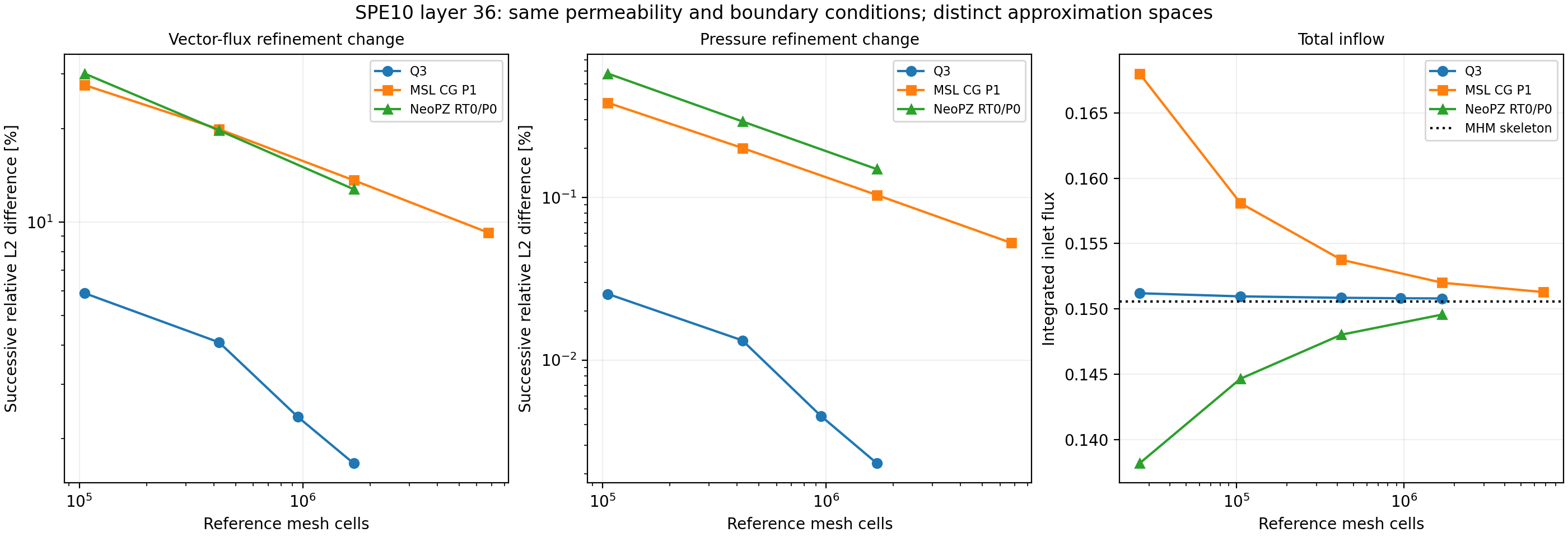
Reference refinement changes and total inflow for Q3, MSL P1 and NeoPZ RT0/P0

The final Q3 step refines each coordinate by 4/3, whereas the MSL and NeoPZ steps double each coordinate. For a doubling comparison, Q3 480×880 to 960×1760 changes by 2.83993% in flux and 0.00681954% in pressure. The terminal 1.66621% change therefore must not be compared as if it used the same refinement ratio as the other two families.

Successive differences measure observed refinement sensitivity; they are not certified errors against the exact reservoir solution. In particular, the terminal MSL and NeoPZ flux changes remain substantial. Their differences from MHM combine the errors of both discrete fields. Agreement of the MHM/Q3 and MHM/MSL percentages alone does not establish that either reference has converged to the exact flux.

Total inflow and conservation

Method	Positive total inflow
MHM skeletal flux	0.1505654992
Conforming Q3, 960×1760	0.1508016962
MSL P1, 960×3520	0.1512890604
NeoPZ RT0/P0, 480×1760	0.1495695509

The sign convention is \(-\int_{y=0}q\cdot n\): upward flow enters at the bottom. For MHM this integral uses the skeletal normal flux. For Q3 and MSL P1 it uses the boundary reactions of the uneliminated variational operator. These reactions need not equal integrals of the raw gradient field on the boundary. For NeoPZ it is the integral of the H(div)-conforming mixed flux itself.

The maximum MHM macro balance defect is \(1.25\times10^{-15}\). NeoPZ has maximum fine-cell balance defect \(5.42\times10^{-18}\), interior normal-flux jump \(6.21\times10^{-18}\), and divergence L2 norm \(1.30\times10^{-16}\). These conservation measurements concern the specified discrete fields; they do not replace the flux-accuracy comparisons.

The direct Q3/RT0 comparison gives 0.132602% pressure difference and 12.3004% vector-flux difference, using the Q3 norms as denominators. Writing \(\mathcal E(q)=\int_\Omega q^{\mathsf T}K^{-1}q\) and \(I\) for positive inflow, the divergence-free RT0 field and prescribed Q3 pressure trace, together with the mixed variational equation, give \(\mathcal E(q_{\mathrm{RT0}})=I_{\mathrm{RT0}}\) and \((K^{-1}q_{\mathrm{Q3}},q_{\mathrm{RT0}})=I_{\mathrm{RT0}}\). The nested RT0 refinements also satisfy \(\mathcal E(q_f-q_c)=I_f-I_c\), with measured relative defects at most \(3.16\times10^{-11}\). For Q3 versus RT0, the directly integrated \(\mathcal E(q_{\mathrm{Q3}}-q_{\mathrm{RT0}})\) is \(1.2321475083\times10^{-3}\), while the archived inlet-reaction difference is \(1.2321452913\times10^{-3}\). Their absolute discrepancy, \(2.22\times10^{-9}\), corresponds to the finite algebraic-work defect between the Q3 energy and its inlet reaction. The resulting relative discrepancy \(1.80\times10^{-6}\) exceeds the recorded \(10^{-7}\) identity criterion, which therefore remains not satisfied. These measurements quantify energy consistency and reaction precision; they are not a certified error bound.

Inspect the records and replay requirements

pixi run --locked -e notebooks gallery-spe10-flux

This command requires the original field archives identified by the comparison record. With those payloads, it reads their coefficients and norms without executing the reference codes. The checkout retains their digests and numerical measurements, rather than all historical full-field arrays. The refinement figure above uses only these retained measurements. Download the case index and aggregated measurements. Integrated comparisons are recorded in darcy-flux-q3-norms.json, msl-cg-mhm-960x3520-q3.json and neopz-mhm-480x1760-order3.json, all in examples/results/spe10. The direct classical-field energy comparison is neopz-q3-480x1760-order7.json, also included in neopz-convergence.json. msl-cg-convergence.json and neopz-provenance.json record reference revisions, solver conventions and artifact digests. The notebook guide includes notebook 23 for inspection of the reservoir results. Reference-code sources and comparison execution programs are not part of this distribution.

References

Gabriel R. Barrenechea, Larissa Martins, Weslley Pereira, and Frédéric Valentin (2026). An H(div; Ω)-Conforming Flux Reconstruction for the Multiscale Hybrid-Mixed Method, Multiscale Modeling & Simulation 24(2), 399–428. DOI: 10.1137/24M1673073.
Diego Paredes, Frédéric Valentin, and Henrique M. Versieux (2024). Revisiting the robustness of the multiscale hybrid-mixed method: The face-based strategy, Journal of Computational and Applied Mathematics 436, 115415. DOI: 10.1016/j.cam.2023.115415.