Mixed Darcy on tetrahedra and prisms

solve_darcy_hdiv3d provides conforming local mixed Darcy solvers on affine tetrahedra and triangular prisms. The skeleton carries physical normal-flux moments on the original macrofaces. Fine interior flux and pressure modes remain independent of the skeletal resolution.

Explicit polynomial families

Let \(P_k\) denote complete total-degree polynomials and \(W_{a,b}=P_a(x,y)\otimes P_b(z)\). The mathematical spaces, rather than a degree label alone, determine the implementation.

Cell	Normal trace	Interior flux construction	Pressure/divergence	Flux dimension
Tetrahedron, `pressure_degree=1`	\(P_1\) on each triangle	\(\{v\in[P_2]^3:v\cdot n\vert_F\in P_1(F)\}\)	\(P_1\)	18: 12 face + 6 interior
Tetrahedron, `pressure_degree=2`	\(P_1\) on each triangle	\(P_1\) face modes and every zero-normal bubble of \([P_3]^3\)	\(P_2\)	32: 12 face + 20 interior
Prism, `pressure_degree=1`	\(P_1\) on triangles, \(Q_1\) on rectangles	Horizontal \(\mathrm{BDFM}_1(\triangle)\otimes P_1(z)\) and vertical \(P_1(x,y)\otimes P_2(z)\)	\(W_{1,1}\)	27: 18 face + 9 interior

The prismatic construction lies in \([W_{2,2}]^3\). The larger space defined only by these normal-trace and divergence constraints has one additional solenoidal bubble; it is not the implemented 27-dimensional tensor construction.

These spaces have been compared with the native TPZShapeHDiv evaluation in NeoPZ. An invertible coefficient transformation is fitted on 150 points and checked on 150 other points. Maximum vector and divergence discrepancies are respectively \(6.14\times10^{-14}\) and \(3.29\times10^{-13}\). The verification record identifies the revision and all three dimensions. Separate native Basix tests check tetrahedral mass/divergence operators and the independent tensor factors of the prism. The runtime does not use NeoPZ coefficients or basis code.

The article's Problem 4 describes tetrahedral BDFM1 while also mentioning quadratic pressure. Those labels do not uniquely specify its internal order. Both compatible choices above are therefore explicit in the API and reported separately. The published prismatic description refers to Castro et al. (2016). Agreement with the recorded NeoPZ revision establishes the executed space; it does not identify the historical revision behind the article's figures.

Interior bubbles use fixed ordered monomial moments and positive-diagonal Cholesky orthonormalization. HDiv3DFamily.coefficients exposes the resulting read-only reference matrix. Persisted solutions store this executed matrix alongside the flux coordinates; field replay uses that matrix for both the oriented face transformation and polynomial evaluation. The records check separate digests for the complete archive and its reference basis.

Piola, boundaries and conservation

For an affine cell map \(F(\hat x)=J\hat x+b\),

\[ q(F(\hat x))=\frac{J\hat q(\hat x)}{\det J},\qquad \nabla\cdot q(F(\hat x))=\frac{\widehat{\nabla\cdot q}(\hat x)}{\det J}. \]

Pressure uses ordinary scalar composition. Since \(\det J\) is constant, the physical divergence and pressure spaces coincide. Normal moment transformations handle both orientation signs and permutations of shared face vertices. Nonaffine prisms are rejected; curved-cell pressure conventions are outside this API. Mapped hexahedra have their own geometry contract.

Pressure Dirichlet values enter the weak boundary load. Neumann data are physical outward normal-flux densities. A pure-Neumann solve retains the joint constant pressure/boundary-potential mode and imposes one physical volume mean. The constitutive, divergence and prescribed-flux blocks each satisfy the stated \(10^{-10}\) backward-error check. Fine-cell conservation tests every pressure moment, including the constant.

The example helpers below are repository sources, supplied separately from the installed library. Open the corresponding notebook to acquire its verified companion, as described in the notebook guide.

from pymhm import AffineMixedMesh
from examples.formulations.application import hdiv_darcy as solve_darcy_hdiv3d

mesh = AffineMixedMesh.unit_cube(kind="prism")
solution = solve_darcy_hdiv3d(
    mesh,
    local_refinement=2,
    dirichlet=lambda x: 1 + x[:, 0] + 2*x[:, 1] + 3*x[:, 2],
)

Setting trace_degree=1 and subdivisions=local_refinement supplies every fine normal moment. Tests compare this condensed representation against a separately assembled uncondensed conforming mixed system. Lower skeletal resolution is an MHM restriction, not an independent classical reference.

Dupuit–Thiem well and geometry

The physical parameters are those of Durán et al. (2019) Problem 4: inner/outer radii \(0.2/50\) m, height 10 m, permeability \(10^{-13}\) m², viscosity \(10^{-3}\) Pa s, outer pressure 25 MPa and production rate \(0.01\) m³/s. The exact pressure and Darcy flux are

\[ p(r)=p_e+\frac{Q\eta}{2\pi\kappa H}\log(r/r_e),\qquad q(x,y,z)=-\frac{Q}{2\pi H}\frac{(x,y,0)}{x^2+y^2}. \]

All three geometries partition the same planar octagonal annulus, with four logarithmically spaced radial bands. Splitting a hexahedral extrusion into two prisms and each prism into three tetrahedra preserves the physical boundary and volume. Further refinement preserves that domain. The pressure boundary data evaluate the exact radial function at points on the polygonal walls; replacing them by the values at a constant circular radius would change the PDE. Both horizontal caps have zero outward flux.

The graded connectivity is original and explicitly recorded. This is a same-domain assessment of the mixed formulations, not a reproduction of unavailable historical meshes or digitized Figure 15 ratios. Volume mass and divergence use positive order-5 rules; boundary pressure uses order 12. Error norms are computed separately with orders 7 and 10. Pressure and vector flux errors are physical volume \(L^2\) norms, divided by the corresponding exact norm. The pressure denominator includes the 25 MPa datum; it is not the norm of the pressure increment. The hexahedral curve reuses the independently recorded RT1/Q1 study with this same pressure normalization. The affine triangular subdivisions and the trilinear hexahedral spaces are different discretizations on the same physical domain. A common refinement factor does not imply equal cell counts or equal computational work across these families.

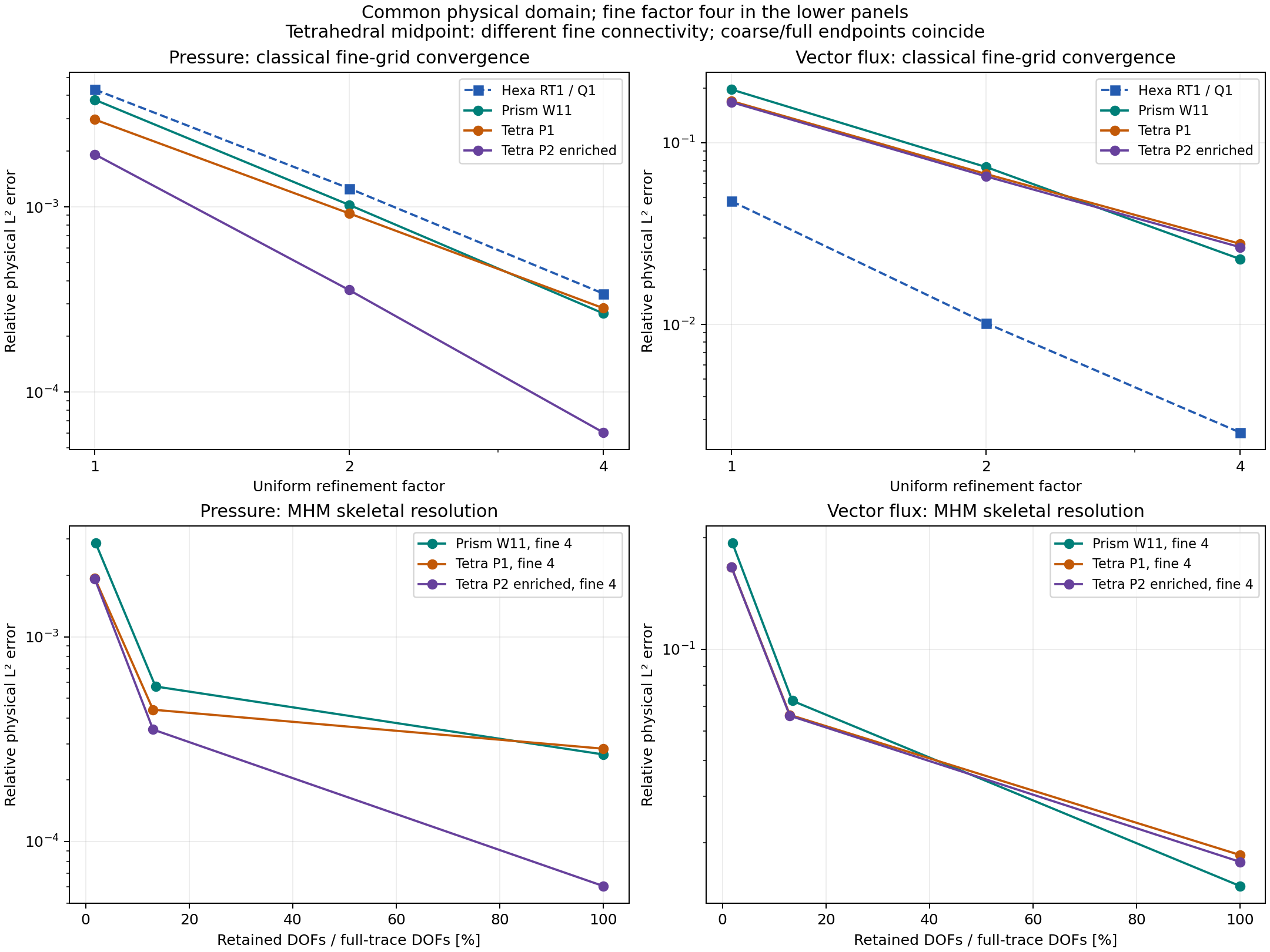
Classical refinement and independent skeletal resolution

The classical limits give the following errors. Refinement factors 1, 2 and 4 refer to subdivision of the same base geometry; all entries are percentages.

Family	Fine cells at factor 4	Flux, factor 1	Flux, factor 2	Flux, factor 4	Pressure, factor 4
Hexahedral RT1/Q1	2,048	4.7694%	1.0174%	0.25409%	0.034040%
Prismatic 27-mode/W11	4,096	19.6410%	7.35818%	2.28985%	0.026611%
Tetrahedral 18-mode/P1	12,288	16.9682%	6.73571%	2.77770%	0.028389%
Tetrahedral 32-mode/P2	12,288	16.7277%	6.53693%	2.66195%	0.006059%

All three affine families reduce both physical errors under classical refinement. On the finest tetrahedral grid, interior enrichment reduces pressure error by a factor of 4.69, while the flux improvement is smaller: both families retain degree-one normal traces. These measurements do not establish an asymptotic order or a universal ranking across geometries and meshes.

The upper panels measure classical spatial refinement. The lower panels use fine factor four and vary the macro partition until every fine trace is retained. The prismatic fine cells are identical throughout. For tetrahedra, the coarsest and finest macro configurations have identical fine cells, but the intermediate composition of two factor-two refinements chooses different internal tetrahedral diagonals. That midpoint therefore combines a skeletal change with a fine-connectivity change. A finer local mesh alone need not remove coarse-trace error. These three operations—local refinement, skeletal resolution, and pressure-space enrichment—remain separate in the records.

The article uses a different ordinate in Figure 15:

\[ \rho_q=\frac{\lVert q-q_{\mathrm{MHM}}\rVert_{L^2(\Omega)}} {\lVert q-q_{\mathrm{classical,fine}}\rVert_{L^2(\Omega)}}. \]

This is the error relative to the classical approximation error, rather than relative to the norm of the exact flux. A value of one means that the MHM error has reached that classical error. The paper by Durán et al. (2019) fixes the fine mesh at H/8 and varies the macro partition; the present affine study reaches factor four on its explicitly declared geometry. Its ratios therefore assess the same approximation mechanism, without reproducing the historical mesh or its Figure 15 values. The pressure and flux profiles in Figure 14 of Durán et al. (2019) use hexahedra, not tetrahedra or prisms.

At fine factor four, the errors for increasing macro resolution are:

Family	Flux error, macro factor 1	Macro factor 2	Macro factor 4	Pressure error, macro factors 1 → 4
Prismatic 27-mode/W11	19.3672%	7.25650%	2.28985%	0.286802% → 0.026611%
Tetrahedral 18-mode/P1	16.6713%	6.64604%	2.77770%	0.193605% → 0.028389%
Tetrahedral 32-mode/P2	16.6625%	6.61069%	2.66195%	0.192001% → 0.006059%

The coarse-trace flux error remains around 17–19% despite local refinement. Interior pressure enrichment alone does not remove it. Across the 18 affine cases, the largest physical block residual is \(1.92\times10^{-13}\) and the largest fine pressure-moment conservation defect is \(1.52\times10^{-17}\) m³/s. Changing error quadrature from order 7 to 10 changes a recorded norm by at most \(9.71\times10^{-6}\) relatively. These checks concern the declared discrete systems and integrations; they are separate from the approximation errors above.

At fine factor four the coarse/full-trace flux-error ratios are approximately 8.46 for prisms, 6.00 for tetrahedral P1 pressure, and 6.26 for tetrahedral P2 pressure. The coarsest skeletal approximation is therefore insufficient for a precise flux field in this well. Small pressure errors and accurate integrated production do not change that conclusion.

The fine-space comparison integrates both solutions on identical physical fine cells. With constant scalar permeability, Galerkin orthogonality gives the flux-error decomposition

\[ \begin{aligned} \lVert q-q_{\mathrm{MHM}}\rVert_{L^2}^2 &=\lVert q-q_f\rVert_{L^2}^2 +\lVert q_f-q_{\mathrm{MHM}}\rVert_{L^2}^2,\\ (q-q_f,\;q_f-q_{\mathrm{MHM}})_{L^2}&=0, \end{aligned} \]

where \(q_f\) is the full-trace classical field. Order-10 integration verifies the squared-norm identity to a relative defect below \(6.14\times10^{-13}\) for the two prismatic restrictions and the coarse/full tetrahedral endpoints. The coarse/full differences, divided by the exact flux norm, are 19.2313%, 16.4383% and 16.4485% for prism, tetrahedral P1 and tetrahedral P2 pressure. This isolates the large skeletal restriction error from the smaller classical fine-space error. The tetrahedral midpoint is excluded from this identity check because its fine connectivity differs.

The same record also reports pressure errors relative to the exact drawdown \(p-p_e\). For the coarsest prismatic skeleton, this error is 5.840%, compared with 0.542% in the full-trace space. The corresponding total-pressure errors are 0.287% and 0.0266%; the outer pressure datum makes those smaller percentages unsuitable for assessing drawdown accuracy by themselves.

The integrated boundary rates are obtained from the archived constant normal moments, with outward signs. The exact rates are \(+0.01\) m³/s at the inner wall, \(-0.01\) m³/s at the exterior, and zero through the horizontal caps. The rate is a diagnostic of the pressure boundary problem, not an additional imposed flux condition. The finest classical inner rates are 0.00999488, 0.00999257 and 0.00999315 m³/s for prism/W11, tetrahedron/P1 and tetrahedron/P2, respectively. The maximum net exterior rate over the 18 cases is below \(1.22\times10^{-17}\) m³/s.

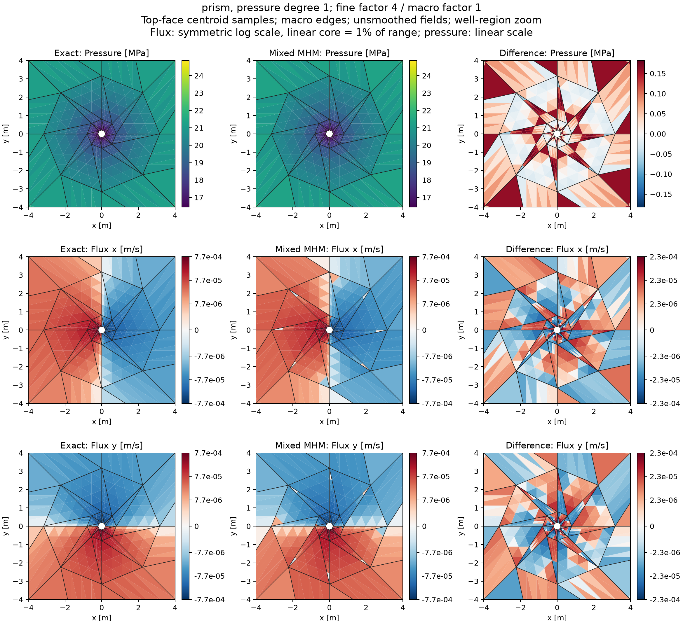
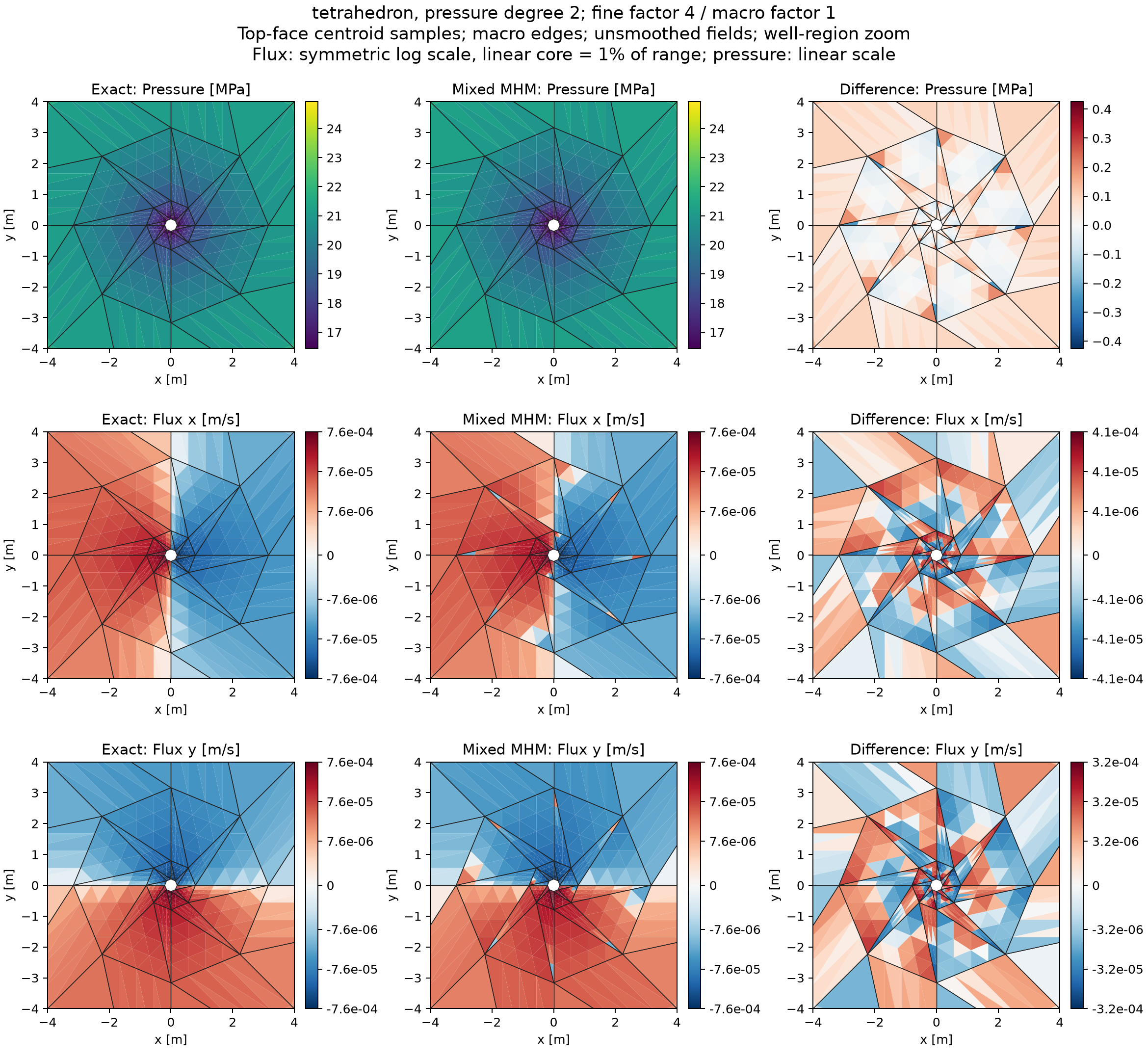
The following maps retain the coarsest macro partition and refine each local cell by factor four. They expose the coarse-trace approximation, rather than showing the full-trace classical limit. The values are one-sided top-face centroid samples without smoothing. Exact and numerical panels use the same sample points and color limits; difference and flux-component scales are centered at zero. Flux panels use a symmetric logarithmic scale, with a linear interval of radius 1% of the displayed absolute limit around zero; no values are clipped. Each difference panel uses its own full symmetric range. Pressure panels remain linear. Black lines are the actual macro edges. The view is restricted to the well neighborhood.

The maps compare the analytical field, the coarse-skeleton MHM field and their signed difference. The physical errors in the tables are volume integrals, rather than norms of top-face display samples. Recorded independent surface quadrature gives coarse/full top-cap flux errors of 19.367%/2.290% for prisms, 22.113%/3.551% for tetrahedral P1 pressure, and 22.085%/3.374% for tetrahedral P2 pressure. A tetrahedral discrete solution need not be invariant in the vertical direction, even though the analytical field is. Surface and volume errors therefore need not coincide. The replay verification checks that evaluating each archived field under different native thread counts preserves its physical values.

The following panels include pressure and signed differences for the coarsest skeletal configuration, with fine factor four and macro factor one. The field replay receipt identifies the coefficient and executed-basis digests, verifies the source records and reports independently integrated norms. Both the oriented face transformation and physical field evaluation use each archive's stored basis matrix. The error panels use their own full color ranges.

Prismatic pressure and signed flux components

Tetrahedral P2 pressure and signed flux components

Independent NeoPZ solution comparison

The reference implementation is NeoPZ 4c6b6d277ce097b97bfc8dea1b6725860f4fe05a, using its native H(div) elements and TPZMixedDarcyFlow material. Classical mixed solves compare the three polynomial families on identical physical cells, first with affine pressure and then with the nonpolynomial well solution. The comparison evaluates physical fields at common quadrature points; it does not equate coefficients belonging to different bases.

NeoPZ also provides the native TPZMHMixedMeshControl implementation. Its own face restrictions define the coarse normal-trace space. For the comparison, the internal and skeletal orders are both one; the 32-mode tetrahedral family additionally enriches the interior by one order. The native controller retains local unknowns in an uncondensed assembled system, while PyMHM condenses them. This compares the same variational restriction using different algebraic resolutions, not parallel performance. No externally imposed restriction matrix replaces the native MHM controller.

Six classical comparisons and six native MHM comparisons cover an affine pressure patch and the well for each polynomial family. All MHM comparisons subdivide each macrocell into eight fine cells, keeping one degree-one trace space per macroface. In the well, the measured relative physical-field differences are:

Family	Macro/fine cells	Flux difference / NeoPZ flux norm	Pressure difference / NeoPZ drawdown norm
Prism, 27 modes/W11	64 / 512	\(3.995\times10^{-12}\)	\(6.037\times10^{-12}\)
Tetrahedron, 18 modes/P1	192 / 1,536	\(2.315\times10^{-12}\)	\(9.998\times10^{-14}\)
Tetrahedron, 32 modes/P2	192 / 1,536	\(2.970\times10^{-12}\)	\(1.482\times10^{-13}\)

The prismatic well, affine patches and classical cases use native NeoPZ skyline LDLᵀ. The two tetrahedral MHM wells use SciPy SuperLU with pivoting and symmetric equilibration on the matrix assembled by NeoPZ. Their coefficients are imported back into NeoPZ for field evaluation and verification against the original unscaled equations. The largest original-system relative residual in the three MHM well cases is \(2.69\times10^{-14}\). This establishes a comparison of native MHM discretizations; it does not attribute SuperLU to NeoPZ.

Both implementations eliminate the prescribed zero normal flux on the caps. Pressure data are integrated on the actual polygonal walls. The solution-verification record identifies the executed cases, quadrature, field norms, code revision and source digests. Agreement between the two implementations is separate from their error relative to the analytical solution: a coarse skeletal space can give the same inaccurate flux in both codes.

Reproduction

pixi run --locked -e test-core python -m examples.solve_mixed_well_geometries --kind prism --fine-factor 4 --macro-factor 1 --workers 4
pixi run --locked -e test-core python -m examples.solve_mixed_well_geometries --kind tetrahedron --pressure-degree 2 --fine-factor 4 --macro-factor 1 --workers 4
pixi run --locked -e notebooks python -m examples.plot_mixed_well_geometries
pixi run --locked -e test-core python -m examples.verify_mixed_well_fields

51_mixed_well_geometries.ipynb executes a small physical patch and reads the recorded campaigns. Acquisition times are concurrent scientific-run metadata, not controlled parallel benchmarks. The recorded elapsed_s covers assembly, condensation, global solution and field reconstruction; the subsequent error-norm integrations are excluded. The acquisition driver requests extended precision for global defect corrections; it therefore requires a platform on which NumPy longdouble has more precision than float64. The solver's default double-precision path and the notebook patch do not impose that requirement. The package supports affine tetrahedra and prisms here; no mixed pyramidal or curved-prism implementation is implied.

References

Douglas A. Castro, Philippe R.B. Devloo, Agnaldo M. Farias, Sônia M. Gomes, Denise de Siqueira, and Omar Durán (2016). Three dimensional hierarchical mixed finite element approximations with enhanced primal variable accuracy. Computer Methods in Applied Mechanics and Engineering 306 479-502. DOI: 10.1016/j.cma.2016.03.050.
Omar Durán, Philippe R. B. Devloo, Sônia M. Gomes, and Frédéric Valentin (2019). A multiscale hybrid method for Darcy’s problems using mixed finite element local solvers, Computer Methods in Applied Mechanics and Engineering 354, 213–244. DOI: 10.1016/j.cma.2019.05.013.